Getting Started with UStatDecouple
Dany Mukesha
2026-01-15
Source:vignettes/getting-started.Rmd
getting-started.RmdAbstract
This vignette provides a gentle introduction to the UStatDecouple package, covering the basic workflow, creating custom kernels, and understanding the output.
1. Installation
# Install from Bioconductor
if (!require("BiocManager", quietly = TRUE))
    install.packages("BiocManager")
BiocManager::install("UStatDecouple")

# Or install the development version
if (!require("remotes", quietly = TRUE))
    install.packages("remotes")
remotes::install_github("dany-mukesha/UStatDecouple")
Load the package:
2. Basic Workflow
The UStatDecouple package follows a simple 4-step workflow:
- Prepare your data as a list of observations
- Create a kernel function that measures similarity/distance between two observations
-
Run decoupling analysis using
decouple_u_stat() -
Interpret the results using the
DecoupleResultobject
Step 1: Prepare Your Data
Your data should be structured as a list, where each element represents one observation (e.g., a DNA sequence, gene expression profile, or any other data type).
# Example: Numeric vectors
data_numeric <- list(
  sample1 = c(1, 3, 5, 7, 9),
  sample2 = c(2, 4, 6, 8, 10),
  sample3 = c(1.5, 3.5, 5.5, 7.5, 9.5),
  sample4 = c(0, 2, 4, 6, 8)
)

# Example: Character vectors (like DNA sequences)
data_dna <- list(
  seq1 = c("A", "C", "G", "T", "A"),
  seq2 = c("A", "C", "G", "T", "C"),
  seq3 = c("A", "C", "G", "A", "A"),
  seq4 = c("T", "C", "G", "T", "A")
)
Step 2: Create a Kernel Function
A kernel function takes two observations and returns a single numeric value representing their similarity or distance.
# Example: Euclidean distance kernel
euclidean_kernel <- function(x, y) {
  sqrt(sum((x - y)^2))
}

# Example: Absolute difference kernel
abs_diff_kernel <- function(x, y) {
  sum(abs(x - y))
}

# Example: Simple matching for sequences (1 if match, 0 if not)
simple_match_kernel <- function(seq1, seq2) {
  sum(seq1 == seq2)
}
Step 3: Run Decoupling Analysis
Use decouple_u_stat() to perform the decoupling
analysis:
# Create a kernel object with metadata
kernel <- create_kernel(euclidean_kernel, "Euclidean Distance")

# Run decoupling
set.seed(123)
result <- decouple_u_stat(
  x = data_numeric,
  kernel = kernel,
  B = 500,  # Number of decoupling iterations
  seed = 123
)
Parameters:
-
x: Your data as a list -
kernel: A UStatKernel object (created withcreate_kernel()) or a plain function -
B: Number of decoupling iterations (higher = more accurate, default: 1000) -
parallel: Use parallel processing (default: FALSE) -
seed: Random seed for reproducibility
Step 4: Interpret the Results
The DecoupleResult object contains several
components:
# Print the result
result
#> DecoupleResult object:
#>   Original U-statistic: 2.4224
#>   Decoupled mean: 1.5746
#>   Decoupled SD: 0.6252
#>   Kernel: Euclidean Distance
#>   Method: Friedman-de la Pena Decoupling
#>   P-value: 0.1751
#>   Z-score: 1.3561
#>   Significance:   (p = 0.1751)

# Access individual components
cat(sprintf("Original statistic: %.4f\n", result@original_stat))
#> Original statistic: 2.4224
cat(sprintf("Decoupled mean: %.4f\n", mean(result@decoupled_distribution)))
#> Decoupled mean: 1.5746
cat(sprintf("Decoupled SD: %.4f\n", sd(result@decoupled_distribution)))
#> Decoupled SD: 0.6252
cat(sprintf("P-value: %.4f\n", result@p_value))
#> P-value: 0.1751
cat(sprintf("Method: %s\n", result@method))
#> Method: Friedman-de la Pena Decoupling
Understanding the output:
- @original_stat: The average of the kernel function evaluated on all pairs in your original data
- @decoupled_distribution: A vector of B values representing what the statistic would be if your data points were independent
- @p_value: Probability of observing a statistic as extreme as yours under independence (two-tailed test)
- @method: The decoupling method used
A low p-value (< 0.05) suggests that your data has dependence structure beyond what would be expected by chance.
3. Visualizing Results
Use the built-in plot() method to visualize the
decoupling distribution:
plot(result, main = "Euclidean Distance Analysis")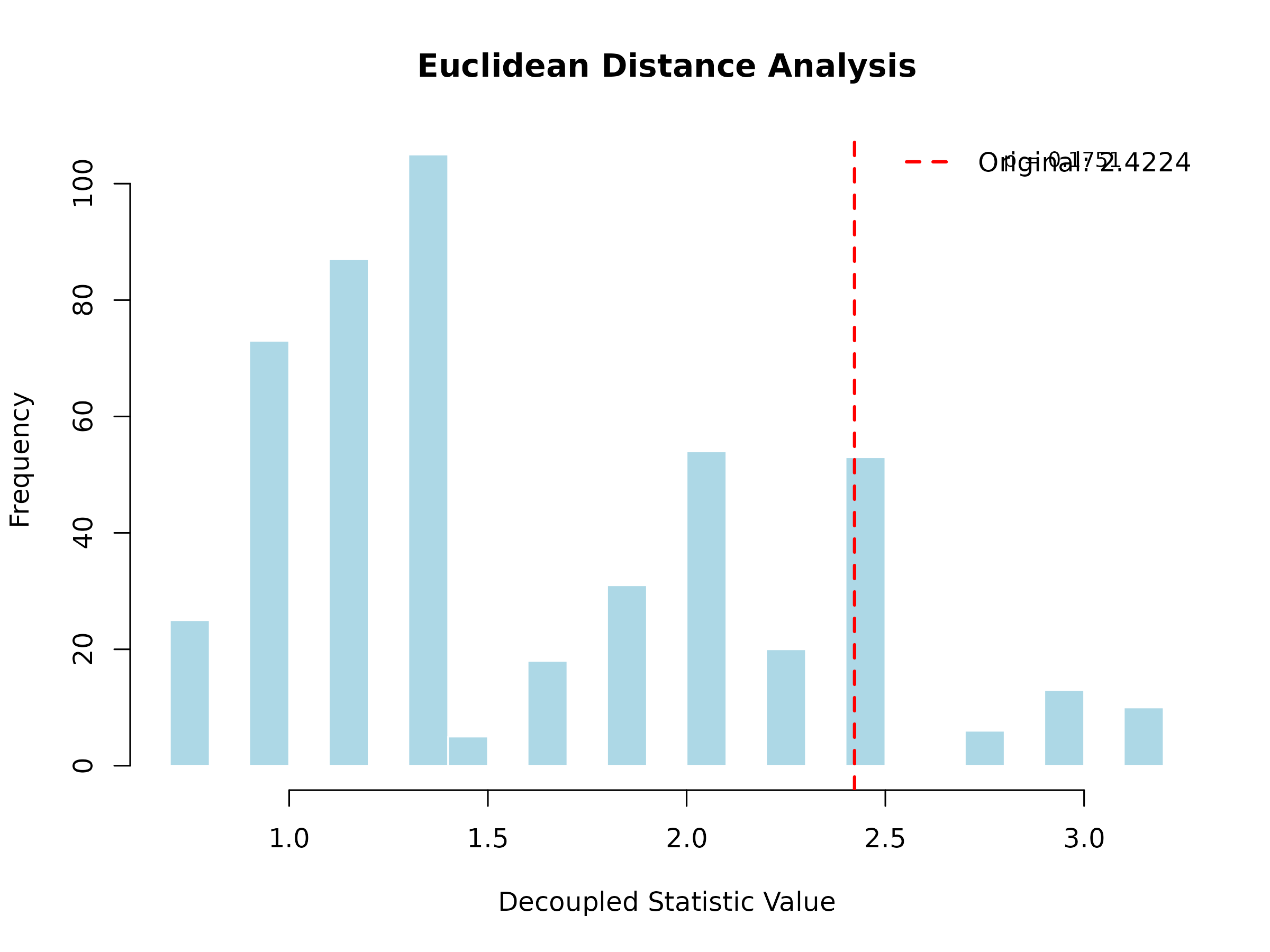
The histogram shows the decoupled distribution (what to expect under independence), and the red vertical line shows the observed statistic. If the observed value falls in the tails of the distribution, this indicates significant dependence.
4. Creating Custom Kernels
You can create any custom kernel function. Here are some examples:
Example 1: Cosine Similarity Kernel
cosine_similarity <- function(x, y) {
  dot_product <- sum(x * y)
  norm_x <- sqrt(sum(x^2))
  norm_y <- sqrt(sum(y^2))
  dot_product / (norm_x * norm_y)
}

# Use it
cosine_kernel <- create_kernel(cosine_similarity, "Cosine Similarity")
cosine_result <- decouple_u_stat(data_numeric, cosine_kernel, B = 200, seed = 123)
plot(cosine_result, main = "Cosine Similarity Analysis")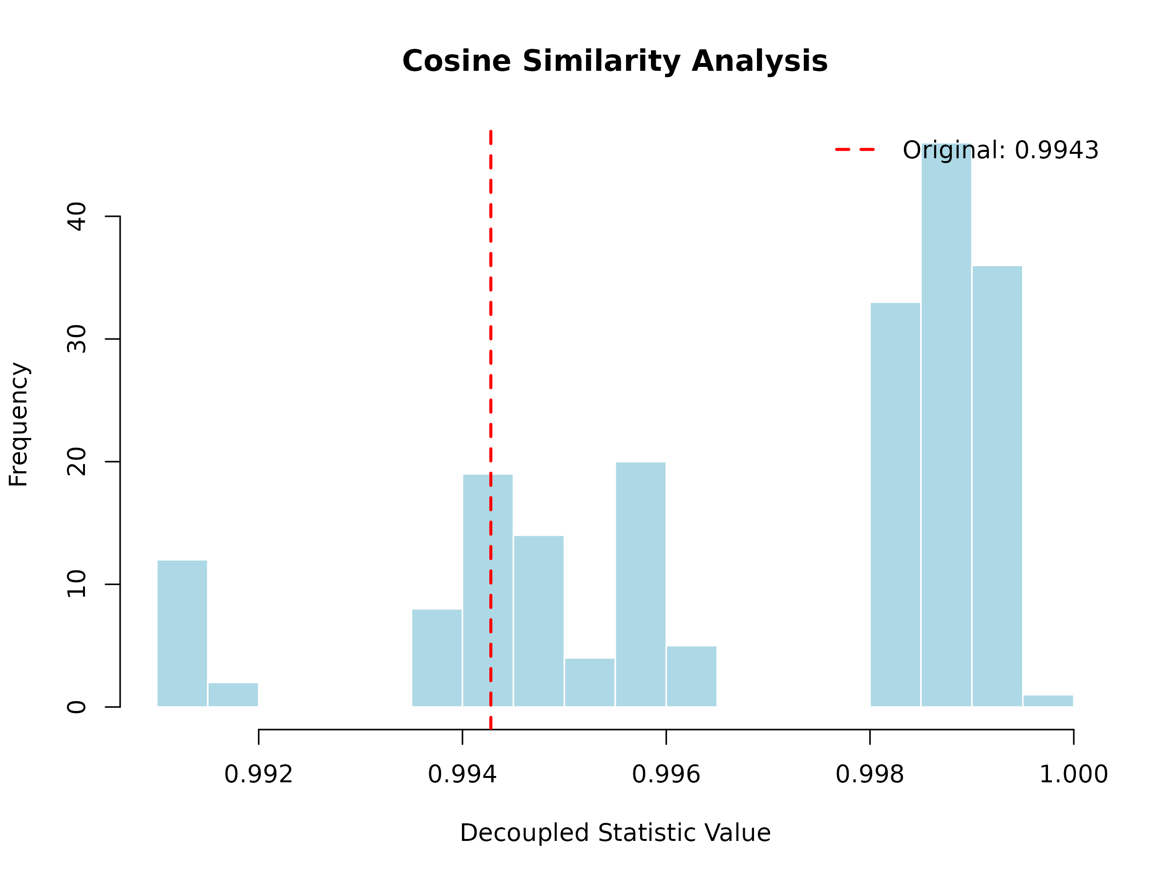
Example 2: Pearson Correlation Kernel
pearson_correlation <- function(x, y) {
  cor(x, y, method = "pearson")
}

# Use it
pearson_kernel <- create_kernel(pearson_correlation, "Pearson Correlation")
pearson_result <- decouple_u_stat(data_numeric, pearson_kernel, B = 200, seed = 123)
plot(pearson_result, main = "Pearson Correlation Analysis")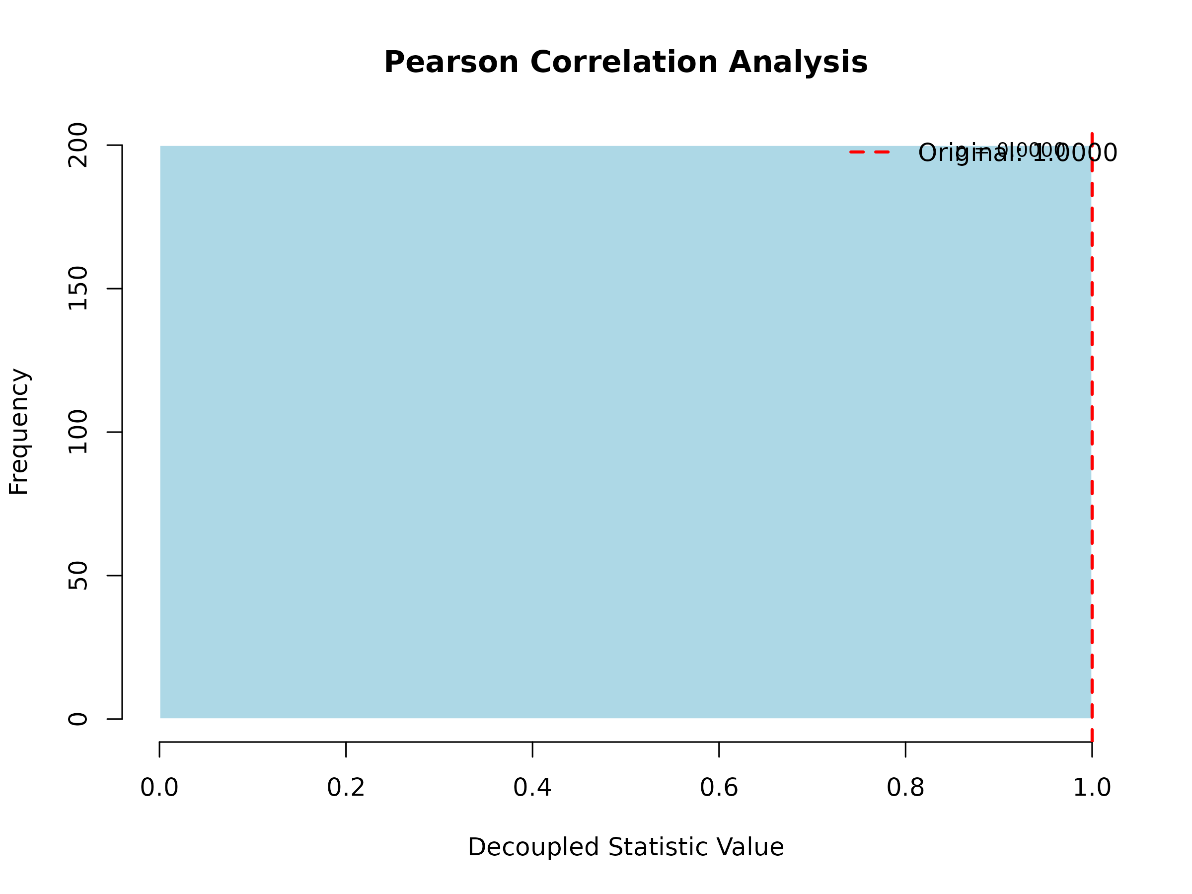
Example 3: Weighted Distance Kernel
# A distance kernel that weights the first half of the vector more heavily
weighted_distance <- function(x, y, weights = NULL) {
  if (is.null(weights)) {
    n <- length(x)
    weights <- c(rep(2, n/2), rep(1, n - n/2))  # First half double weight
  }
  sqrt(sum(weights * (x - y)^2))
}

# Use it
weighted_kernel <- create_kernel(weighted_distance, "Weighted Distance")
weighted_result <- decouple_u_stat(data_numeric, weighted_kernel, B = 200, seed = 123)
plot(weighted_result, main = "Weighted Distance Analysis")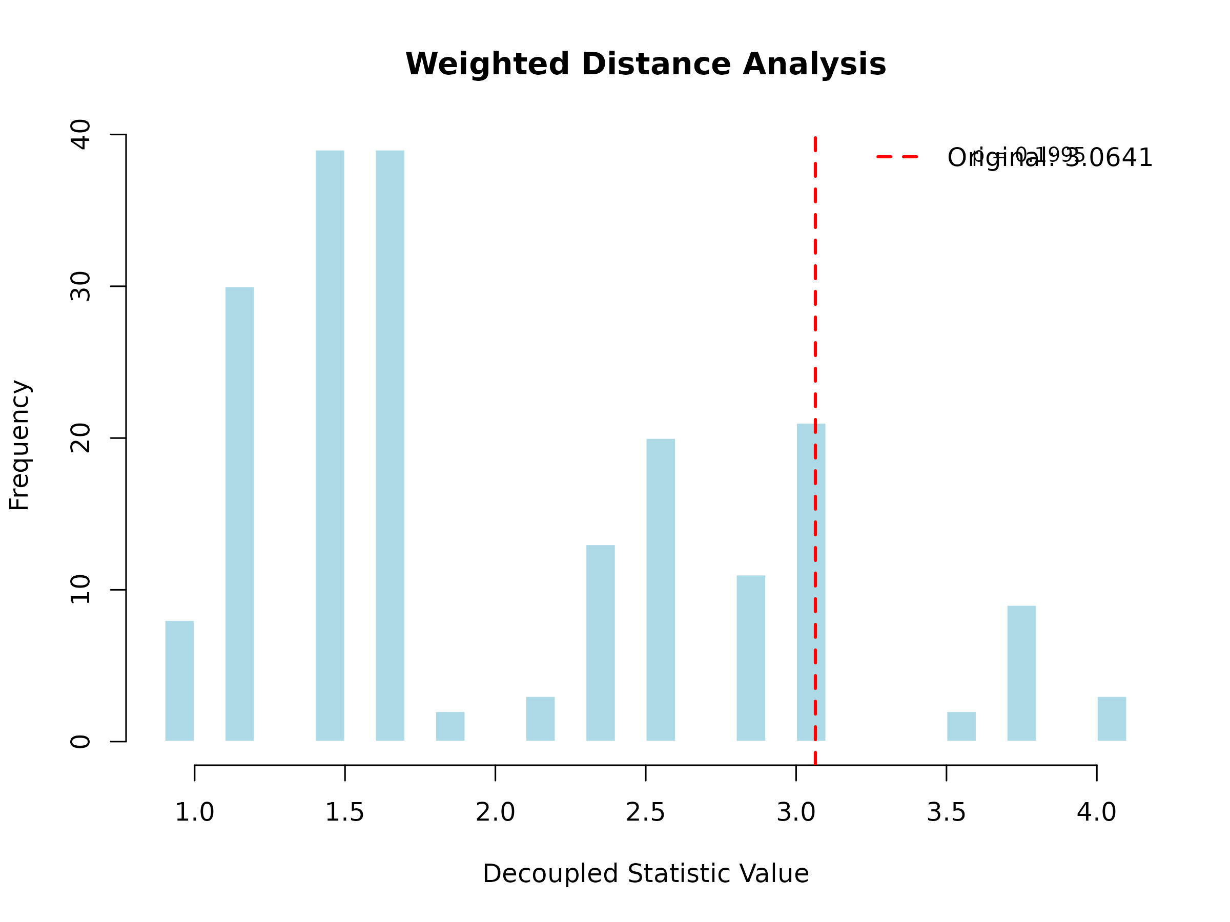
Example 4: Kernel with Multiple Arguments
If your kernel needs additional parameters, create a wrapper function:
# A kernel with a customizable parameter
custom_distance <- function(alpha = 1) {
  function(x, y) {
    (sum(abs(x - y)^alpha))^(1/alpha)
  }
}

# Create kernel with alpha = 2 (Euclidean-like)
euclidean_like <- create_kernel(custom_distance(alpha = 2), "Minkowski (α=2)")
result1 <- decouple_u_stat(data_numeric, euclidean_like, B = 200, seed = 123)

# Create kernel with alpha = 1 (Manhattan-like)
manhattan_like <- create_kernel(custom_distance(alpha = 1), "Minkowski (α=1)")
result2 <- decouple_u_stat(data_numeric, manhattan_like, B = 200, seed = 123)

# Compare
cat(sprintf("α=2 p-value: %.4f\n", result1@p_value))
#> α=2 p-value: 0.1995
cat(sprintf("α=1 p-value: %.4f\n", result2@p_value))
#> α=1 p-value: 0.1995
5. Understanding P-Values
The p-value is calculated using a two-tailed test based on the decoupled distribution:
# The p-value calculation
null_mean <- mean(result@decoupled_distribution)
null_sd <- sd(result@decoupled_distribution)
z_score <- (result@original_stat - null_mean) / null_sd
p_value <- 2 * (1 - pnorm(abs(z_score)))

cat(sprintf("Z-score: %.4f\n", z_score))
#> Z-score: 1.3561
cat(sprintf("P-value: %.4f\n", p_value))
#> P-value: 0.1751
Interpretation:
- p < 0.05: Strong evidence of dependence
- p < 0.01: Very strong evidence of dependence
- p < 0.001: Extremely strong evidence of dependence
- p ≥ 0.05: No significant evidence of dependence
6. Choosing the Right Kernel
The choice of kernel depends on your data and research question:
| Data Type | Suggested Kernel | What it Measures |
|---|---|---|
| Numeric vectors | Euclidean distance, Correlation | Geometric distance, linear relationship |
| Sequences | Hamming distance | Number of differing positions |
| Gene expression | Absolute correlation | Co-expression strength |
| Categorical | Jaccard index, Matching coefficient | Set similarity |
| Time series | Dynamic Time Warping distance | Temporal alignment |
7. Performance Tips
For larger datasets:
# Use parallel processing
large_result <- decouple_u_stat(
  x = large_data,
  kernel = my_kernel,
  B = 1000,
  parallel = TRUE  # Enables parallel computation
)

# Reduce B for faster (but less accurate) results
quick_result <- decouple_u_stat(
  x = data,
  kernel = my_kernel,
  B = 100  # Fewer iterations = faster
)
8. Common Errors and Solutions
Error: “Sample size must be at least 2”
# Wrong: Single observation
bad_data <- list(x = c(1, 2, 3))
decouple_u_stat(bad_data, kernel)  # Error!

# Correct: Multiple observations
good_data <- list(
  x = c(1, 2, 3),
  y = c(4, 5, 6)
)
decouple_u_stat(good_data, kernel)  # Works!
Error: “Kernel must be either a UStatKernel object or a function”
# Wrong: Passing a string
decouple_u_stat(data, "euclidean")  # Error!

# Correct: Create a kernel object
kernel <- create_kernel(euclidean_kernel, "Euclidean")
decouple_u_stat(data, kernel) # Works!9. Next Steps
Now that you understand the basics, you can:
- Explore biological applications: See the main vignette for genomic case studies
- Try with your own data: Apply the workflow to your research data
- Experiment with custom kernels: Design kernels specific to your domain
- Compare multiple kernels: Test different kernels to see which best captures your dependence structure
For more advanced topics and biological applications, see the main
UStatDecouple vignette.