Genetic Algorithm Optimization • genetic.algo.optimizeR

The goal of genetic.algo.optimizeR is to optimize the function f(x) = x² − 4x + 4 using a genetic algorithm. The function represents a simple quadratic equation, and the goal is to find the value of x that minimizes the function.

Here’s a breakdown of the aim and the results:

Aim:

Optimize the function f(x) = x² − 4x + 4 to find the value of x that minimizes the function.

Results:

Initial Population:
- We start with a population of three individuals: x₁ = 1, x₂ = 3, and x₃ = 0.
Evaluation:
- We evaluate the fitness of each individual by calculating f(x) for each x value:
  - f(1) = 1² − 4 * 1 + 4 = 1
  - f(3) = 3² − 4 * 3 + 4 = 1
  - f(0) = 0² − 4 * 0 + 4 = 4
Selection:
- We select individuals x₁ and x₂ as parents for crossover because they have higher fitness.
Crossover and Mutation:
- We perform crossover and mutation on the selected parents to generate offspring: x₁′ = 1, x₂′ = 3.
Replacement:
- We replace individual x₃ with offspring x₁′, maintaining the population size.

After multiple generations of repeating these steps, the genetic algorithm aims to converge towards an optimal or near-optimal solution. In this example, since it’s simple and the solution space is small, we could expect the algorithm to converge relatively quickly towards the optimal solution x = 2, where f(x) = 0.

Explaining Graph Web capture_8-2-2024_233215_mermaid live

Usage

library(genetic.algo.optimizeR)

# Initialize population
population <- initialize_population(population_size = 3, min = 0, max = 3)
print("Initial Population:")
#> [1] "Initial Population:"
print(population)
#> [1] 0 1 3

generation <- 0 # Initialize generation/reputation counter

while (TRUE) {
  generation <- generation + 1 # Increment generation/reputation count

  # Evaluate fitness
  fitness <- evaluate_fitness(population)
  print("Evaluation:")
  print(fitness)


  # Check if the fitness of every individual is close to zero
  if (all(abs(fitness) <= 0.01)) {
    print("Termination Condition Reached: All individuals have fitness close to zero.")
    break
  }

  # Selection
  selected_parents <- selection(population, fitness, num_parents = 2)
  print("Selection:")
  print(selected_parents)

  # Crossover and Mutation
  offspring <- crossover(selected_parents, offspring_size = 2)
  mutated_offspring <- mutation(offspring, mutation_rate = 0) # (no mutation in this example)
  print("Crossover and Mutation:")
  print(mutated_offspring)

  # Replacement
  population <- replacement(population, mutated_offspring, num_to_replace = 1)
  print("Replacement:")
  print(population)
}
#> [1] "Evaluation:"
#> [1] 4 1 1
#> [1] "Selection:"
#> [1] 1 3
#> [1] "Crossover and Mutation:"
#> [1] 2 2
#> [1] "Replacement:"
#> [1] 0 1 2
#> [1] "Evaluation:"
#> [1] 4 1 0
#> [1] "Selection:"
#> [1] 2 1
#> [1] "Crossover and Mutation:"
#> [1] 2 2
#> [1] "Replacement:"
#> [1] 2 1 2
#> [1] "Evaluation:"
#> [1] 0 1 0
#> [1] "Selection:"
#> [1] 2 2
#> [1] "Crossover and Mutation:"
#> [1] 2 2
#> [1] "Replacement:"
#> [1] 2 2 2
#> [1] "Evaluation:"
#> [1] 0 0 0
#> [1] "Termination Condition Reached: All individuals have fitness close to zero."

print(paste("Total generations/reputations:", generation))
#> [1] "Total generations/reputations: 4"

The above example illustrates the process of a genetic algorithm, where individuals are selected, crossed over, and replaced iteratively to improve the population towards finding the optimal solution(i.e. fitting population).

In theory

Initialize Population:
- Start with a population of individuals: X1(x=1), X2(x=3), X3(x=0).
  (Note: the values are random and the population should be highly diversified)
- The space of x value is kept integer type and on range from 0 to 3,for simplification.
```
population <- c(1, 3, 0)
population
#> [1] 1 3 0
```
Evaluate Fitness:
- Calculate fitness(f(x)) for each individual:
  - X1: f(1) = 1^2 - 4*1 + 4 = 1
  - X2: f(3) = 3^2 - 4*3 + 4 = 1
  - X3: f(0) = 0^2 - 4*0 + 4 = 4

Coding the function f(x) in R A quadratic function is a function of the form: ax2+bx+c where a≠0

So for:

f(x) = x² − 4x + 4

In R, we write:

a <- 1
b <- -4
c <- 4
f <- function(x) {
  a * x^2 + b * x + c
}

Plotting the quadratic function f(x) First, we have to choose a domain over which we want to plot f(x).

Let’s try 0 ≤ x ≤ 3:

# domain over which we want to plot f(x)
x <- seq(from = 0, to = 4, length.out = 100)
# plot f(x)
plot(x, f(x), type = "l") # type = 'l' plots a line instead of points
# plot the x and y axes
abline(v = 0, h = 0, col = "skyblue", lty = 3)
points(c(1, 3), c(f(1), f(3)), col = "coral1", pch = 8, cex = 1.5, lty = 3)
text(c(1, 3), c(f(1), f(3)), labels = c("(x=1, f(x=1))", "(x=3, f(x=3))"), pos = 3)

points(c(0), c(f(0)), col = "blue", pch = 8, cex = 1.5, lty = 3)
text(c(0), c(f(0)), labels = "(x=0, f(x=0))", pos = 4, font = 2)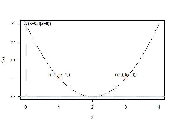

Selection:
- Select parents for crossover:
  - Y1(x=1), Y2(x=3)

# plot f(x)
plot(x, f(x), type = "l") # type = 'l' plots a line instead of points
# plot the x and y axes
points(c(1, 3), c(f(1), f(3)), col = "coral1", pch = 8, cex = 2, lty = 3)
text(c(1, 3), c(f(1), f(3)), labels = c("(x=1, f(x=1))", "(x=3, f(x=3))"), pos = 3, font = 2)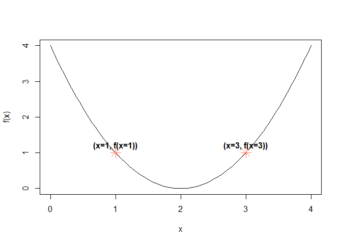

Crossover and Mutation:
- Generate offspring through crossover and mutation:
  - Z1(x=1), Z2(x=3) (no mutation in this example)
Replacement:
- Replace individuals in the population:
  - Replace X3 with Z1, maintaining the population size.
Repeat Steps 2-5 for multiple generations until a termination condition is met.

The optimal/fitting individuals F of a quadratic equation, in this case the lowest point on the graph of f(x), is:

$$ F\left(\frac{-b}{2a}, f\left(\frac{-b}{2a}\right)\right) $$

find.fitting <- function(a, b, c) {
  x_fitting <- -b / (2 * a)
  y_fitting <- f(x_fitting)
  c(x_fitting, y_fitting)
}
F <- find.fitting(a, b, c)

Adding the Fitting to the plot:

# plot f(x)
plot(x, f(x), type = "l") # type = 'l' plots a line instead of points
# plot the x and y axes
abline(h = 0)
abline(v = 0)
# add the vertex to the plot
points(
  x = F[1], y = F[2],
  pch = 18, cex = 2, col = "red"
) # pch controls the form of the point and cex controls its size
# add a label next to the point
text(
  x = F[1], y = F[2],
  labels = "Fitting", pos = 3, col = "red", font = 10
) # pos = 3 places the text above the point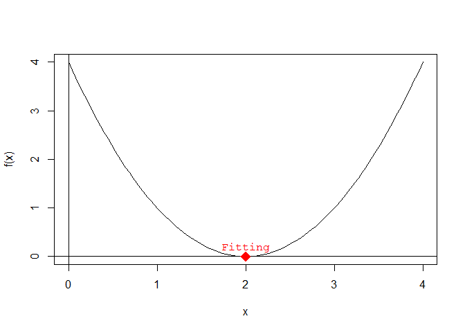

Existing alternative solution

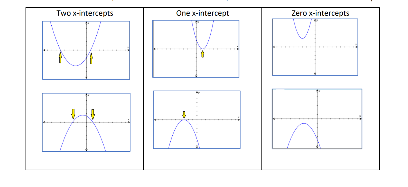
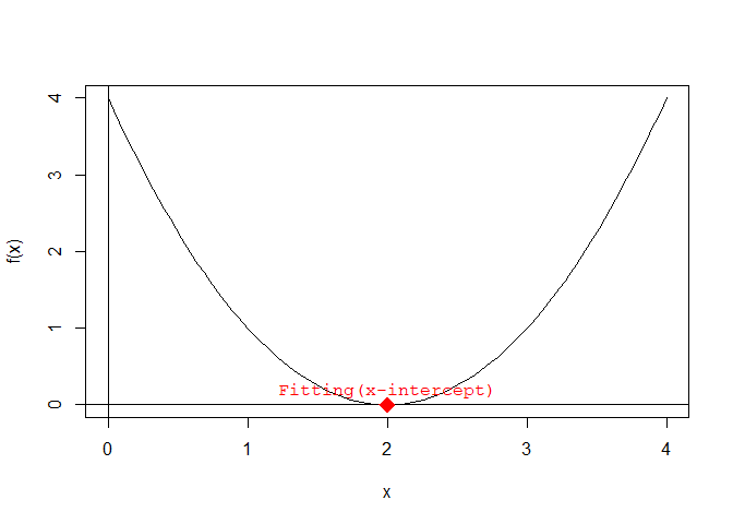
Finding the x-intercepts of f(x)

The x-intercepts are the solutions of the quadratic equation f(x) = 0; they can be found by using the quadratic formula:

$$ x = \frac{-b \pm \sqrt{b^2 - 4ac}}{2a} $$

The quantity b2–4ac is called the discriminant:

if the discriminant is positive, then f(x) has 2 solutions (i.e. x-intercepts).
if the discriminant is zero, then f(x) has 1 solution (i.e. 1 x-intercept).
if the discriminant is negative, then f(x) has no real solutions (i.e. does not intersect the x-axis).

# find the x-intercepts of f(x)
find.roots <- function(a, b, c) {
  discriminant <- b^2 - 4 * a * c
  if (discriminant > 0) {
    c((-b - sqrt(discriminant)) / (2 * a), (-b + sqrt(discriminant)) / (2 * a))
  } else if (discriminant == 0) {
    -b / (2 * a)
  } else {
    NaN
  }
}
solutions <- find.roots(a, b, c)

Adding the x-intercepts to the plot:

# plot f(x)
plot(x, f(x), type = "l") # type = 'l' plots a line instead of points
# plot the x and y axes
abline(h = 0)
abline(v = 0)
# add the x-intercepts to the plot
points(
  x = solutions, y = rep(0, length(solutions)), # x and y coordinates of the x-intercepts
  pch = 18, cex = 2, col = "red"
)
text(
  x = solutions, y = rep(0, length(solutions)),
  labels = rep("Fitting(x-intercept)", length(solutions)),
  pos = 3, col = "red", font = 10
)

{genetic.algo.optimizeR}

Usage

References

- Goldberg, D. E. (1989). Genetic Algorithms in Search, Optimization and Machine Learning. Addison-Wesley.
- Holland, J. H. (1992). Adaptation in Natural and Artificial Systems. MIT Press.
- Whitley, D. (1994). A genetic algorithm tutorial. Statistics and Computing, 4(2), 65-85
- Deb, K., Pratap, A., Agarwal, S., & Meyarivan, T. A. M. T. (2002). A fast and elitist multiobjective genetic algorithm: NSGA-II. IEEE Transactions on Evolutionary Computation, 6(2), 182-197.