Theory

Theory

1. Initialize Population:
   • Start with a population of individuals: X1(x=1), X2(x=3), X3(x=0).
     (Note: the values are random and the population should be highly diversified)
   • The space of x value is kept integer type and on range from 0 to 3,for simplification.

population <- c(1, 3, 0)

2. Evaluate Fitness:

   • Calculate fitness(f(x)) for each individual:

     • X1: f(1) = 1^2 - 4*1 + 4 = 1
     • X2: f(3) = 3^2 - 4*3 + 4 = 1
     • X3: f(0) = 0^2 - 4*0 + 4 = 4

     Coding the function f(x) in R A quadratic function is a function of the form: ax2+bx+c where a≠0

     So for\(f(x) = x^2 - 4x + 4\)

In R, we write:

a <- 1
b <- -4
c <- 4
f <- function(x) {
    a * x^2 + b * x + c
}

Plotting the quadratic function f(x) First, we have to choose a domain over which we want to plot f(x).

Let’s try 0 ≤ x ≤ 3:

# Define the domain over which we want to plot f(x)
x <- seq(from = 0, to = 4, length.out = 100)

# Define the domain over which we want to plot f(x) and create df data frame
df <- x |>
    data.frame(x = _) |>
    dplyr::mutate(y = f(x))

# Define the space over which we want to population to be
possible_xvalues <- seq(from = 0, to = 3, length.out = 4)

# Create space data frame
space <- possible_xvalues |>
    data.frame(x = _) |>
    dplyr::mutate(y = f(x))

# Calculate fitness inline
fitness <- population^2 - 4 * population + 4

# Selected the surviving parents
num_parents <- 2
selected_parents <- population |>
    order(fitness, decreasing = FALSE) |>
    head(num_parents)

# Plot f(x) using ggplot
ggplot2::ggplot(df, aes(x = x, y = y)) +
    geom_line(color = "black") + # Plot the function as a line
    geom_point(data = subset(space, x %in% c(1, 3)), color = "coral1", size = 3, shape = 8) + # Plot points at x=1 and x=3
    geom_point(data = subset(space, (x == 0)), color = "blue", size = 3, shape = 8) + # Plot a point at x=0
    geom_hline(yintercept = 0, linetype = "dashed", color = "blue") + # Add horizontal line at y=0
    geom_vline(xintercept = 0, linetype = "dashed", color = "blue") + # Add vertical line at x=0
    theme_minimal()

3. Selection:

   • Select parents for crossover:

     • Y1(x=1), Y2(x=3)

# Plot f(x) using ggplot
ggplot(df, aes(x = x, y = y)) +
    geom_line(color = "black") + # Plot the function as a line
    geom_point(data = subset(space, x %in% c(1, 3)), color = "coral1", size = 6, shape = 8) + # Plot points at x=1 and x=3
    geom_hline(yintercept = 0, linetype = "dashed", color = "blue") + # Add horizontal line at y=0
    geom_vline(xintercept = 0, linetype = "dashed", color = "blue") + # Add vertical line at x=0
    theme_minimal() # Use a minimal theme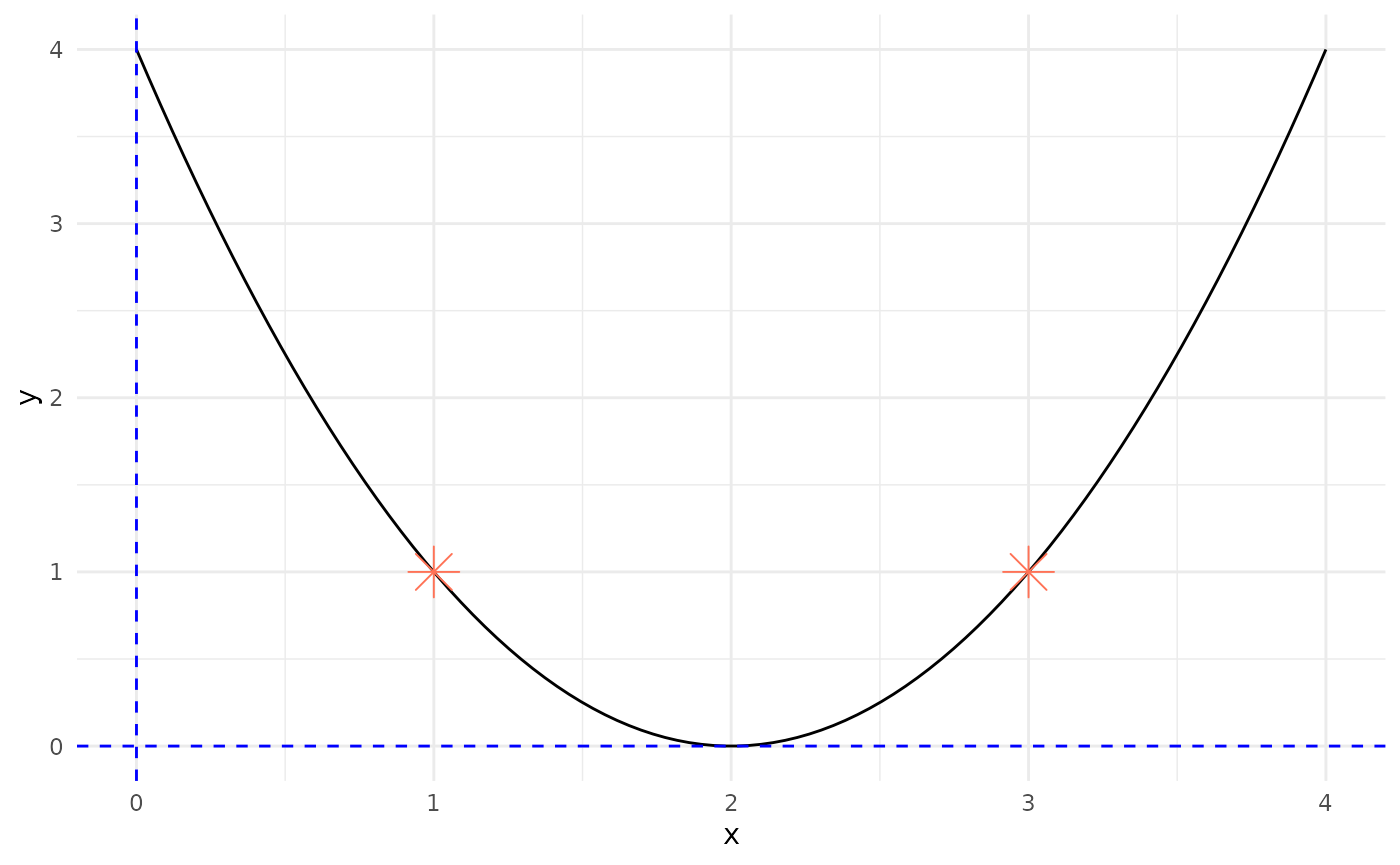

4. Crossover and Mutation:
   • Generate offspring through crossover and mutation:
     • Z1(x=1), Z2(x=3) (no mutation in this example)
5. Replacement:
   • Replace individuals in the population:
     • Replace X3 with Z1, maintaining the population size.
6. Repeat Steps 2-5 for multiple generations until a termination condition is met.

The optimal/fitting individuals F of a quadratic equation, in this case the lowest point on the graph of f(x), is:

\[ F\left(\frac{-b}{2a}, f\left(\frac{-b}{2a}\right)\right) \]

find.fitting <- function(a, b, c) {
    x_fitting <- -b / (2 * a)
    y_fitting <- f(x_fitting)
    c(x_fitting, y_fitting)
}
F <- find.fitting(a, b, c)

Adding the Fitting to the plot:

# Plot f(x) using ggplot
ggplot(df, aes(x = x, y = y)) +
    geom_line(color = "black") + # Plot the function as a line
    geom_hline(yintercept = 0, linetype = "dashed") + # Add horizontal line at y=0
    geom_vline(xintercept = 0, linetype = "dashed") + # Add vertical line at x=0
    geom_point(x = F[1], y = F[2], shape = 18, size = 6, color = "red") + # Plot the vertex
    geom_text(x = F[1], y = F[2], label = "Fitting", vjust = -1, color = "red", size = 5) + # Add label next to the vertex
    theme_minimal() # Use a minimal theme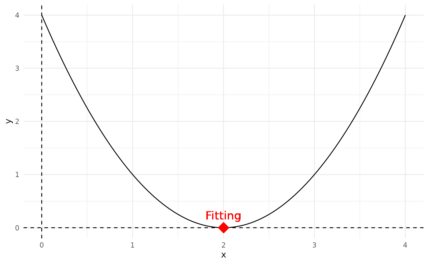

Existing alternative solution

Finding the x-intercepts of f(x)

The x-intercepts are the solutions of the quadratic equation f(x) = 0; they can be found by using the quadratic formula:

\[ x = \frac{-b \pm \sqrt{b^2 - 4ac}}{2a} \]

The quantity \(b2–4ac\) is called the discriminant:

• if the discriminant is positive, then f(x) has 2 solutions (i.e. x-intercepts).
• if the discriminant is zero, then f(x) has 1 solution (i.e. 1 x-intercept).
• if the discriminant is negative, then f(x) has no real solutions (i.e. does not intersect the x-axis).

# find the x-intercepts of f(x)
find.roots <- function(a, b, c) {
    discriminant <- b^2 - 4 * a * c
    if (discriminant > 0) {
        c((-b - sqrt(discriminant)) / (2 * a), (-b + sqrt(discriminant)) / (2 * a))
    } else if (discriminant == 0) {
        -b / (2 * a)
    } else {
        NaN
    }
}
solutions <- find.roots(a, b, c)

Adding the x-intercepts to the plot:

# Plot f(x) using ggplot
ggplot(df, aes(x = x, y = y)) +
    geom_line(color = "black") + # Plot the function as a line
    geom_hline(yintercept = 0, linetype = "dashed") + # Add horizontal line at y=0
    geom_vline(xintercept = 0, linetype = "dashed") + # Add vertical line at x=0
    geom_point(data = data.frame(x = solutions, y = rep(0, length(solutions))), shape = 18, size = 6, color = "red") + # Plot x-intercepts
    geom_text(data = data.frame(x = solutions, y = rep(0, length(solutions)), label = "Fitting(x-intercept)"), aes(label = label), vjust = -1, color = "red", size = 5) + # Add labels next to x-intercepts
    theme_minimal() # Use a minimal theme