Introduction to TCMC
Dany Mukesha
Université Côte d’Azurdanymukesha@gmail.com
26 November 2024
Source:vignettes/TCMC.Rmd
TCMC.RmdAbstract
Machine learning model selection is a critical step in the development of predictive analytics projects. We introduce TCMC, an R package made to streamline the process of comparing and selecting classification models. TCMC facilitates the evaluation of 13 diverse classification algorithms using the caret package, providing users with a clean framework for model assessment. TCMC implements a powerful methodology, including repeated cross-validation for performance estimation and the generation of variable importance plots. The package supports customizable training/test split ratios and produces confusion matrices for detailed model evaluation. The primary metric of TCMC for comparison is accuracy, but it also enables the calculation of additional metrics such as sensitivity, specificity, and F1 score. We demonstrate the utility of package using the Pima Indians Diabetes dataset, comparing models such as Learning Vector Quantization (LVQ), Gradient Boosting Machine (GBM), Support Vector Machine (SVM), and Random Forest (RF), more others. The results showcase the ability of package to efficiently train multiple models and provide clear comparisons of their performance. TCMC addresses the need for a standardized, reproducible approach to model selection in classification tasks. By automating the comparison process and providing detailed performance metrics, it enables the user to make informed decisions about model selection, potentially improving the overall quality of predictive models in various domains. This tool contributes to the field of machine learning by offering a user-friendly, extensible platform for model comparison, suitable for both research and practical applications in data science and predictive analytics.Basics
Install TCMC
TCMC package (Mukesha, 2024) will be soon available on Bioconductor.
if (!requireNamespace("BiocManager", quietly = TRUE)) {
    install.packages("BiocManager")
}
BiocManager::install("TCMC")
BiocManager::valid()
Citing TCMC
I hope that TCMC will be useful for research. Please use the following information to cite the package and the overall approach. Thank you!
citation("TCMC")
#> To cite package 'TCMC' in publications use:
#>
#>   Mukesha D (2024). _TCMC: Compare Classification Models_. R package
#>   version 0.99.0, https://danymukesha.github.io/TCMC/,
#>   <https://github.com/danymukesha/TCMC>.
#>
#> A BibTeX entry for LaTeX users is
#>
#>   @Manual{,
#>     title = {TCMC: Compare Classification Models},
#>     author = {Dany Mukesha},
#>     year = {2024},
#>     note = {R package version 0.99.0,
#> https://danymukesha.github.io/TCMC/},
#>     url = {https://github.com/danymukesha/TCMC},
#>   }
Quick start to using TCMC
data(PimaIndiansDiabetes)
str(PimaIndiansDiabetes)
#> 'data.frame':    768 obs. of  9 variables:
#>  $ pregnant: num  6 1 8 1 0 5 3 10 2 8 ...
#>  $ glucose : num  148 85 183 89 137 116 78 115 197 125 ...
#>  $ pressure: num  72 66 64 66 40 74 50 0 70 96 ...
#>  $ triceps : num  35 29 0 23 35 0 32 0 45 0 ...
#>  $ insulin : num  0 0 0 94 168 0 88 0 543 0 ...
#>  $ mass    : num  33.6 26.6 23.3 28.1 43.1 25.6 31 35.3 30.5 0 ...
#>  $ pedigree: num  0.627 0.351 0.672 0.167 2.288 ...
#>  $ age     : num  50 31 32 21 33 30 26 29 53 54 ...
#>  $ diabetes: Factor w/ 2 levels "neg","pos": 2 1 2 1 2 1 2 1 2 2 ...
# for this example only LVQ and GBM are being tested
results <- model_comparer(PimaIndiansDiabetes, "diabetes", for_utest = TRUE)
# plot variable importance for a specific model
plot_importance(results$trained_models$lvq, "LVQ")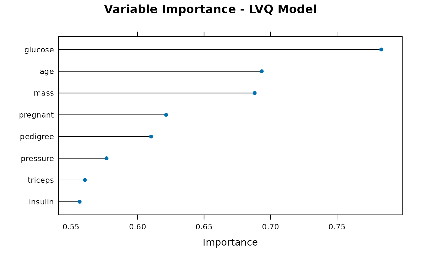
plot_importance(results$trained_models$rf, "RF")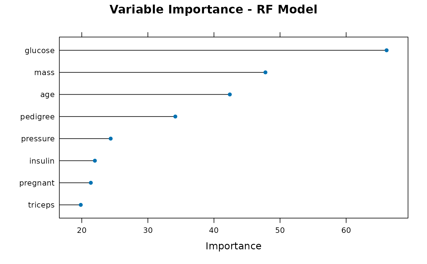
# access trained models
models_results <- resamples(results$trained_models)
summary(models_results)
#>
#> Call:
#> summary.resamples(object = models_results)
#>
#> Models: lvq, rf
#> Number of resamples: 30
#>
#> Accuracy
#>          Min.   1st Qu.    Median      Mean   3rd Qu.      Max. NA's
#> lvq 0.5806452 0.6935484 0.7096774 0.7041953 0.7246827 0.8032787    0
#> rf  0.6612903 0.7377049 0.7704918 0.7669663 0.8056584 0.8709677    0
#>
#> Kappa
#>          Min.   1st Qu.    Median      Mean   3rd Qu.      Max. NA's
#> lvq 0.0450237 0.2567240 0.3124786 0.3010701 0.3747960 0.5436409    0
#> rf  0.2203593 0.3655972 0.4799026 0.4738476 0.5648847 0.7181818    0
bwplot(models_results)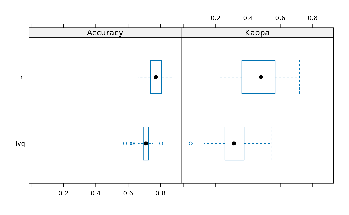
best_model <- results$performance$rf
best_model
#> Confusion Matrix and Statistics
#>
#>           Reference
#> Prediction pos neg
#>        pos  33  20
#>        neg  16  84
#>
#>                Accuracy : 0.7647
#>                  95% CI : (0.6894, 0.8294)
#>     No Information Rate : 0.6797
#>     P-Value [Acc > NIR] : 0.01348
#>
#>                   Kappa : 0.471
#>
#>  Mcnemar's Test P-Value : 0.61708
#>
#>             Sensitivity : 0.6735
#>             Specificity : 0.8077
#>          Pos Pred Value : 0.6226
#>          Neg Pred Value : 0.8400
#>              Prevalence : 0.3203
#>          Detection Rate : 0.2157
#>    Detection Prevalence : 0.3464
#>       Balanced Accuracy : 0.7406
#>
#>        'Positive' Class : pos
#>
Example with SummarizedExperiment
Example integrated with SummarizedExperiment (Morgan, Obenchain, Hester, and Pagès, 2024) with machine learning workflows for evaluating treatment effectiveness.
Scenario description: In this example, we investigate the effectiveness of different treatments in influencing positive outcomes for a simulated clinical dataset. Each treatment corresponds to a class of drugs (e.g., TZD and DPP-4), and the outcome variable indicates whether the response to treatment was positive or negative. Using the SummarizedExperiment (Morgan, Obenchain, Hester et al., 2024) class from Bioconductor, we will preprocess the data, train machine learning models, and analyze the most impactful features and models.
Data simulation: The dataset contains measurements of sugar levels across eight samples, along with metadata describing treatment classes and outcomes. The SummarizedExperiment (Morgan, Obenchain, Hester et al., 2024) object is used to organize and manage this data.
library(SummarizedExperiment)

# Simulate data
nrows <- 200 # Number of features (e.g., genes or biomarkers)
ncols <- 8  # Number of samples
sugar_level <- matrix(runif(nrows * ncols, 1, 500), nrows)

# Metadata: treatment classes and outcomes
colData <- DataFrame(Treatment_class = rep(c("TZD", "DPP-4"), 4),
        row.names = LETTERS[1:8])
Outcome <- DataFrame(Outcome = (rep(c("neg", "pos"), 5)))
se0 <- SummarizedExperiment(assays = SimpleList(counts = sugar_level),
        colData = colData, metadata = Outcome)
# in the case the input is a SummarizedExperiment, extract assay and metadata
if (inherits(se0, "SummarizedExperiment")) {
    data <- as.data.frame(assay(se0))
    metadata <- as.data.frame(metadata(se0))
    data_df <- cbind(metadata, data)
}
feature_names <- c("Outcome",
    "TreatmentA", "TreatmentB", "TreatmentC", "TreatmentD",
    "TreatmentE", "TreatmentF", "TreatmentG", "TreatmentH"
)
colnames(data_df) <- feature_names
data_df$Outcome <- data_df$Outcome |> as.factor()
str(data_df)
#> 'data.frame':    200 obs. of  9 variables:
#>  $ Outcome   : Factor w/ 2 levels "neg","pos": 1 2 1 2 1 2 1 2 1 2 ...
#>  $ TreatmentA: num  134.4 497.7 433.6 61.7 205.1 ...
#>  $ TreatmentB: num  244.9 15.4 61.9 372.7 89 ...
#>  $ TreatmentC: num  189 310 331 376 102 ...
#>  $ TreatmentD: num  155 399 216 226 342 ...
#>  $ TreatmentE: num  173 51 270 474 168 ...
#>  $ TreatmentF: num  238.4 313 393.6 28.9 299.4 ...
#>  $ TreatmentG: num  362.1 398.6 44.6 257.1 37.1 ...
#>  $ TreatmentH: num  464.3 128 424.8 51.1 305.8 ...
results <- model_comparer(data = data_df, "Outcome", for_utest = TRUE)
plot_importance(results$trained_models$lvq, "LVQ", type_plot = "enhanced")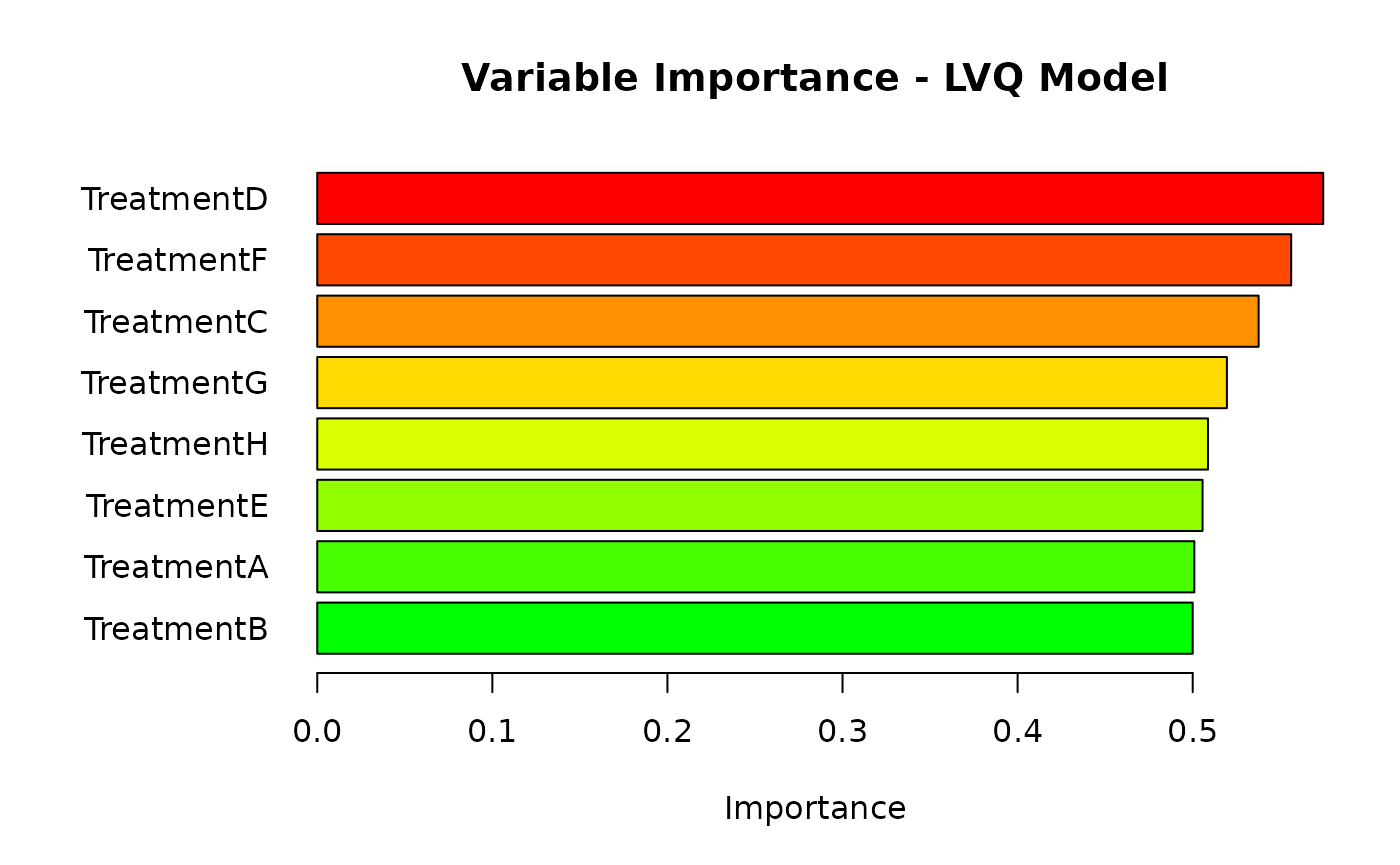
plot_importance(results$trained_models$rf, "RF", type_plot = "basic")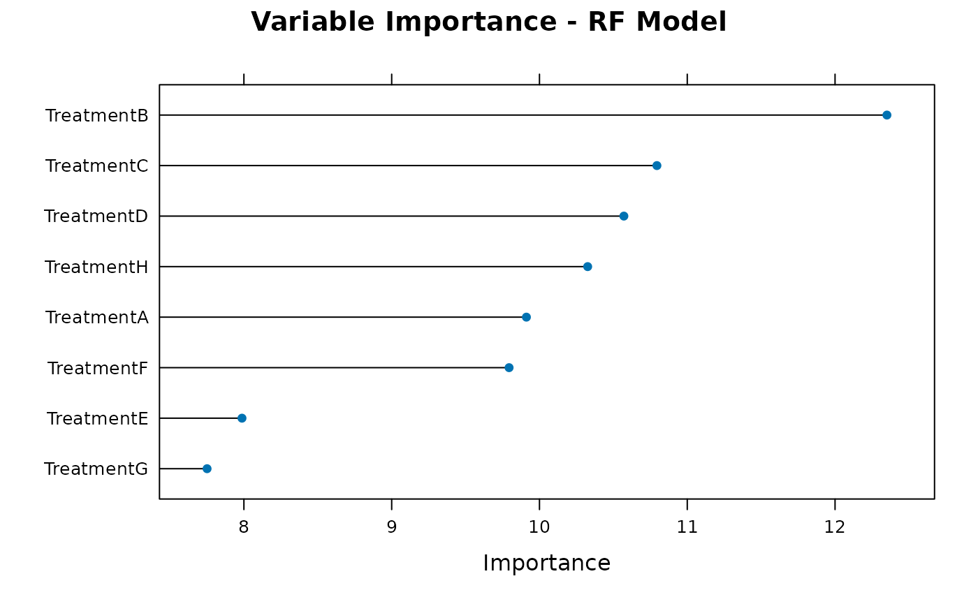
models_results <- resamples(results$trained_models)
summary(models_results)
#>
#> Call:
#> summary.resamples(object = models_results)
#>
#> Models: lvq, rf
#> Number of resamples: 30
#>
#> Accuracy
#>       Min. 1st Qu. Median    Mean  3rd Qu.   Max. NA's
#> lvq 0.2500  0.4375 0.5625 0.52500 0.609375 0.7500    0
#> rf  0.3125  0.4375 0.5000 0.48125 0.546875 0.6875    0
#>
#> Kappa
#>       Min. 1st Qu. Median    Mean 3rd Qu.  Max. NA's
#> lvq -0.500  -0.125  0.125  0.0500 0.21875 0.500    0
#> rf  -0.375  -0.125  0.000 -0.0375 0.09375 0.375    0

bwplot(models_results)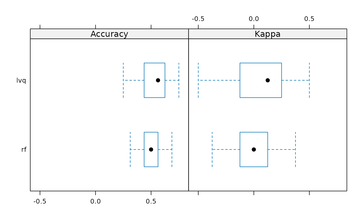
best_model <- results$performance$rf
best_model
#> Confusion Matrix and Statistics
#>
#>           Reference
#> Prediction pos neg
#>        pos   7  13
#>        neg  10  10
#>
#>                Accuracy : 0.425
#>                  95% CI : (0.2704, 0.5911)
#>     No Information Rate : 0.575
#>     P-Value [Acc > NIR] : 0.9806
#>
#>                   Kappa : -0.15
#>
#>  Mcnemar's Test P-Value : 0.6767
#>
#>             Sensitivity : 0.4118
#>             Specificity : 0.4348
#>          Pos Pred Value : 0.3500
#>          Neg Pred Value : 0.5000
#>              Prevalence : 0.4250
#>          Detection Rate : 0.1750
#>    Detection Prevalence : 0.5000
#>       Balanced Accuracy : 0.4233
#>
#>        'Positive' Class : pos
#>
By identifying the most predictive treatments and features, we can inform clinical decision-making and prioritize interventions that maximize positive outcomes.
Here is an example of you can cite your package inside the vignette:
- TCMC (Mukesha, 2024)
The data set utilized in the example is originally from the National Institute of Diabetes and Digestive and Kidney Diseases.
- Source: mlbench (Leisch and Dimitriadou, 2024)
Date the vignette was generated.
#> [1] "2024-11-26 14:36:12 UTC"Wallclock time spent generating the vignette.
#> Time difference of 36.704 secsR session information.
#> ─ Session info ───────────────────────────────────────────────────────────────────────────────────────────────────────
#>  setting  value
#>  version  R version 4.4.2 (2024-10-31)
#>  os       Ubuntu 22.04.5 LTS
#>  system   x86_64, linux-gnu
#>  ui       X11
#>  language en
#>  collate  C.UTF-8
#>  ctype    C.UTF-8
#>  tz       UTC
#>  date     2024-11-26
#>  pandoc   3.1.11 @ /opt/hostedtoolcache/pandoc/3.1.11/x64/ (via rmarkdown)
#>
#> ─ Packages ───────────────────────────────────────────────────────────────────────────────────────────────────────────
#>  package              * version    date (UTC) lib source
#>  abind                  1.4-8      2024-09-12 [1] RSPM
#>  backports              1.5.0      2024-05-23 [1] RSPM
#>  bibtex                 0.5.1      2023-01-26 [1] RSPM
#>  Biobase              * 2.66.0     2024-10-29 [1] Bioconduc~
#>  BiocGenerics         * 0.52.0     2024-10-29 [1] Bioconduc~
#>  BiocManager            1.30.25    2024-08-28 [1] RSPM
#>  BiocStyle            * 2.34.0     2024-10-29 [1] Bioconduc~
#>  bookdown               0.41       2024-10-16 [1] RSPM
#>  bslib                  0.8.0      2024-07-29 [1] RSPM
#>  C50                    0.1.8      2023-02-08 [1] RSPM
#>  cachem                 1.1.0      2024-05-16 [1] RSPM
#>  caret                * 6.0-94     2023-03-21 [1] RSPM
#>  class                  7.3-22     2023-05-03 [3] CRAN (R 4.4.2)
#>  cli                    3.6.3      2024-06-21 [1] RSPM
#>  codetools              0.2-20     2024-03-31 [3] CRAN (R 4.4.2)
#>  colorspace             2.1-1      2024-07-26 [1] RSPM
#>  combinat               0.0-8      2012-10-29 [1] RSPM
#>  crayon                 1.5.3      2024-06-20 [1] RSPM
#>  Cubist                 0.4.4      2024-07-02 [1] RSPM
#>  data.table             1.16.2     2024-10-10 [1] RSPM
#>  DelayedArray           0.32.0     2024-10-29 [1] Bioconduc~
#>  desc                   1.4.3      2023-12-10 [1] RSPM
#>  digest                 0.6.37     2024-08-19 [1] RSPM
#>  dplyr                  1.1.4      2023-11-17 [1] RSPM
#>  e1071                  1.7-16     2024-09-16 [1] RSPM
#>  evaluate               1.0.1      2024-10-10 [1] RSPM
#>  fansi                  1.0.6      2023-12-08 [1] RSPM
#>  fastmap                1.2.0      2024-05-15 [1] RSPM
#>  forcats                1.0.0      2023-01-29 [1] RSPM
#>  foreach                1.5.2      2022-02-02 [1] RSPM
#>  Formula                1.2-5      2023-02-24 [1] RSPM
#>  fs                     1.6.5      2024-10-30 [1] RSPM
#>  future                 1.34.0     2024-07-29 [1] RSPM
#>  future.apply           1.11.3     2024-10-27 [1] RSPM
#>  gbm                    2.2.2      2024-06-28 [1] RSPM
#>  generics               0.1.3      2022-07-05 [1] RSPM
#>  GenomeInfoDb         * 1.42.0     2024-10-29 [1] Bioconduc~
#>  GenomeInfoDbData       1.2.13     2024-11-26 [1] Bioconductor
#>  GenomicRanges        * 1.58.0     2024-10-29 [1] Bioconduc~
#>  ggplot2              * 3.5.1      2024-04-23 [1] RSPM
#>  globals                0.16.3     2024-03-08 [1] RSPM
#>  glue                   1.8.0      2024-09-30 [1] RSPM
#>  gower                  1.0.1      2022-12-22 [1] RSPM
#>  gtable                 0.3.6      2024-10-25 [1] RSPM
#>  hardhat                1.4.0      2024-06-02 [1] RSPM
#>  haven                  2.5.4      2023-11-30 [1] RSPM
#>  highr                  0.11       2024-05-26 [1] RSPM
#>  hms                    1.1.3      2023-03-21 [1] RSPM
#>  htmltools              0.5.8.1    2024-04-04 [1] RSPM
#>  httpuv                 1.6.15     2024-03-26 [1] RSPM
#>  httr                   1.4.7      2023-08-15 [1] RSPM
#>  inum                   1.0-5      2023-03-09 [1] RSPM
#>  ipred                  0.9-15     2024-07-18 [1] RSPM
#>  IRanges              * 2.40.0     2024-10-29 [1] Bioconduc~
#>  iterators              1.0.14     2022-02-05 [1] RSPM
#>  jquerylib              0.1.4      2021-04-26 [1] RSPM
#>  jsonlite               1.8.9      2024-09-20 [1] RSPM
#>  klaR                   1.7-3      2023-12-13 [1] RSPM
#>  knitr                  1.49       2024-11-08 [1] RSPM
#>  labelled               2.13.0     2024-04-23 [1] RSPM
#>  later                  1.3.2      2023-12-06 [1] RSPM
#>  lattice              * 0.22-6     2024-03-20 [3] CRAN (R 4.4.2)
#>  lava                   1.8.0      2024-03-05 [1] RSPM
#>  libcoin                1.0-10     2023-09-27 [1] RSPM
#>  lifecycle              1.0.4      2023-11-07 [1] RSPM
#>  listenv                0.9.1      2024-01-29 [1] RSPM
#>  lubridate              1.9.3      2023-09-27 [1] RSPM
#>  magrittr               2.0.3      2022-03-30 [1] RSPM
#>  MASS                   7.3-61     2024-06-13 [3] CRAN (R 4.4.2)
#>  Matrix                 1.7-1      2024-10-18 [3] CRAN (R 4.4.2)
#>  MatrixGenerics       * 1.18.0     2024-10-29 [1] Bioconduc~
#>  matrixStats          * 1.4.1      2024-09-08 [1] RSPM
#>  mime                   0.12       2021-09-28 [1] RSPM
#>  miniUI                 0.1.1.1    2018-05-18 [1] RSPM
#>  mlbench              * 2.1-5      2024-05-02 [1] RSPM
#>  ModelMetrics           1.2.2.2    2020-03-17 [1] RSPM
#>  munsell                0.5.1      2024-04-01 [1] RSPM
#>  mvtnorm                1.3-2      2024-11-04 [1] RSPM
#>  nlme                   3.1-166    2024-08-14 [3] CRAN (R 4.4.2)
#>  nnet                   7.3-19     2023-05-03 [3] CRAN (R 4.4.2)
#>  parallelly             1.39.0     2024-11-07 [1] RSPM
#>  partykit               1.2-22     2024-08-17 [1] RSPM
#>  pillar                 1.9.0      2023-03-22 [1] RSPM
#>  pkgconfig              2.0.3      2019-09-22 [1] RSPM
#>  pkgdown                2.1.1      2024-09-17 [1] any (@2.1.1)
#>  plyr                   1.8.9      2023-10-02 [1] RSPM
#>  pROC                   1.18.5     2023-11-01 [1] RSPM
#>  prodlim                2024.06.25 2024-06-24 [1] RSPM
#>  promises               1.3.0      2024-04-05 [1] RSPM
#>  proxy                  0.4-27     2022-06-09 [1] RSPM
#>  purrr                  1.0.2      2023-08-10 [1] RSPM
#>  questionr              0.7.8      2023-01-31 [1] RSPM
#>  R6                     2.5.1      2021-08-19 [1] RSPM
#>  ragg                   1.3.3      2024-09-11 [1] RSPM
#>  randomForest           4.7-1.2    2024-09-22 [1] RSPM
#>  Rcpp                   1.0.13-1   2024-11-02 [1] RSPM
#>  recipes                1.1.0      2024-07-04 [1] RSPM
#>  RefManageR           * 1.4.0      2022-09-30 [1] RSPM
#>  reshape2               1.4.4      2020-04-09 [1] RSPM
#>  rlang                  1.1.4      2024-06-04 [1] RSPM
#>  rmarkdown              2.29       2024-11-04 [1] RSPM
#>  rpart                  4.1.23     2023-12-05 [3] CRAN (R 4.4.2)
#>  rstudioapi             0.17.1     2024-10-22 [1] RSPM
#>  S4Arrays               1.6.0      2024-10-29 [1] Bioconduc~
#>  S4Vectors            * 0.44.0     2024-10-29 [1] Bioconduc~
#>  sass                   0.4.9      2024-03-15 [1] RSPM
#>  scales                 1.3.0      2023-11-28 [1] RSPM
#>  sessioninfo          * 1.2.2      2021-12-06 [1] RSPM
#>  shiny                  1.9.1      2024-08-01 [1] RSPM
#>  SparseArray            1.6.0      2024-10-29 [1] Bioconduc~
#>  stringi                1.8.4      2024-05-06 [1] RSPM
#>  stringr                1.5.1      2023-11-14 [1] RSPM
#>  SummarizedExperiment * 1.36.0     2024-10-29 [1] Bioconduc~
#>  survival               3.7-0      2024-06-05 [3] CRAN (R 4.4.2)
#>  systemfonts            1.1.0      2024-05-15 [1] RSPM
#>  TCMC                 * 0.99.0     2024-11-26 [1] local
#>  textshaping            0.4.0      2024-05-24 [1] RSPM
#>  tibble                 3.2.1      2023-03-20 [1] RSPM
#>  tidyselect             1.2.1      2024-03-11 [1] RSPM
#>  tidyverse              2.0.0      2023-02-22 [1] RSPM
#>  timechange             0.3.0      2024-01-18 [1] RSPM
#>  timeDate               4041.110   2024-09-22 [1] RSPM
#>  UCSC.utils             1.2.0      2024-10-29 [1] Bioconduc~
#>  utf8                   1.2.4      2023-10-22 [1] RSPM
#>  vctrs                  0.6.5      2023-12-01 [1] RSPM
#>  withr                  3.0.2      2024-10-28 [1] RSPM
#>  xfun                   0.49       2024-10-31 [1] RSPM
#>  xml2                   1.3.6      2023-12-04 [1] RSPM
#>  xtable                 1.8-4      2019-04-21 [1] RSPM
#>  XVector                0.46.0     2024-10-29 [1] Bioconduc~
#>  yaml                   2.3.10     2024-07-26 [1] RSPM
#>  zlibbioc               1.52.0     2024-10-29 [1] Bioconduc~
#>
#>  [1] /home/runner/work/_temp/Library
#>  [2] /opt/R/4.4.2/lib/R/site-library
#>  [3] /opt/R/4.4.2/lib/R/library
#>
#> ──────────────────────────────────────────────────────────────────────────────────────────────────────────────────────
Bibliography
[1] F. Leisch and E. Dimitriadou. mlbench: Machine Learning Benchmark Problems. R package version 2.1-5. 2024. URL: https://CRAN.R-project.org/package=mlbench.
[2] M. Morgan, V. Obenchain, J. Hester, et al. SummarizedExperiment: A container (S4 class) for matrix-like assays. R package version 1.36.0. 2024. DOI: 10.18129/B9.bioc.SummarizedExperiment. URL: https://bioconductor.org/packages/SummarizedExperiment.
[3] D. Mukesha. TCMC: Compare Classification Models. R package version 0.99.0, https://danymukesha.github.io/TCMC/. 2024. URL: https://github.com/danymukesha/TCMC.