Abstract
Genetic algorithms (GAs) are optimization techniques inspired by the process of natural selection and genetics. They operate by evolving a population of candidate solutions over successive generations, with each individual representing a potential solution to the optimization problem at hand. Through the application of genetic operators such as selection, crossover, and mutation, the genetic algorithms iteratively improve the population by eventually converging towards optimal or near-optimal solutions. In the field of genomics, where data sets are often large, complex, and high-dimensional, the genetic algorithms offer a good approach for addressing optimization challenges such as feature selection, parameter tuning, and model optimization. By harnessing the power of evolutionary principles, genetic algorithms can effectively explore the solution space, identify informative features, and optimize model parameters, leading to improved accuracy and interpretability in genomic data analysis. The BioGA package extends the capabilities of genetic algorithms to the realm of genomic data analysis, providing a suite of functions optimized for handling high throughput genomic data. Implemented in C++ for enhanced performance, BioGA offers efficient algorithms for tasks such as feature selection, classification, clustering, and more. By integrating flawlessly with the Bioconductor ecosystem, BioGA empowers users to take advantage of the power of genetic algorithms within their genomics workflows, facilitating the discovery of biological insights from large-scale genomic data sets.Getting Started
Installation
To install this package, start R (version “4.4”) and enter:
if (!require("BiocManager", quietly = TRUE))
    install.packages("BiocManager")

# The following initializes usage of Bioc devel
BiocManager::install(version='devel')

BiocManager::install(pkgs = "BioGA", version = "devel", force = TRUE)
You can also install the package directly from GitHub using the
devtools package:
devtools::install_github("danymukesha/BioGA")With a simplified example, we illustrated the usage of BioGA for genetic algorithm optimization in the context of high throughput genomic data analysis. We showcased its interoperability with Bioconductor classes, demonstrating how genetic algorithm optimization can be integrated into existing genomics pipelines to improve the analysis and interpretation.
We demonstrated the usage of BioGA in the context of selecting the best combination of genes for predicting a certain trait, such as disease susceptibility.
Implementation
Algorithmic Framework
The core of BioGA lies in a modified version of the NSGA-II algorithm, tailored specifically for the demands of high-throughput genomic data. Traditional implementations of NSGA-II operate on generic problem domains, but BioGA introduces biologically informed heuristics at multiple stages of the evolutionary cycle to better capture the structure of genomic data. From initialization to mutation, each step of the algorithm leverages gene-level relationships to maintain biological plausibility.
A notable innovation is the multi-objective fitness
function, which combines classification accuracy and gene set
sparsity. By adjusting a tunable parameter α, users can
customize the trade-off depending on whether interpretability (fewer
genes) or predictive power is more important for their application. The
fitness evaluation is parallelized using OpenMP, allowing for fast
computation even with large populations and datasets.
The C++ snippet included demonstrates how the fitness evaluation computes three key metrics; accuracy, sparsity, and a weighted combination of both to guide the evolutionary selection. Importantly, this performance-critical computation is written in native C++ with Rcpp, yielding both speed and memory efficiency.
Software Architecture
BioGA’s
layered architecture is designed for modularity, scalability,
and user accessibility. At the top layer, a clean
R/Bioconductor interface makes the tool accessible to the bioinformatics
community, providing standard S4 object support and integration with
SummarizedExperiment and ExpressionSet
classes. This enables seamless incorporation into existing genomic
analysis pipelines.
The middle layer, written in C++ using RcppArmadillo, provides the computational engine. This layer is fully parallelized using RcppParallel and OpenMP, enabling users to exploit multi-core architectures. Even on commodity hardware, BioGA can outperform many existing tools due to this efficient backend.
Finally, the architecture connects with biological databases and annotation frameworks, including STRINGdb, WGCNA, and KEGG pathways. This integration ensures that evolutionary operators such as mutation and selection are biologically informed rather than purely random, which is a critical advancement over traditional GA models that ignore gene-gene relationships.
Biologically Informed Operators
A standout feature of BioGA is its ability to incorporate biological knowledge directly into the evolutionary process. Instead of relying on purely stochastic operations, BioGA uses known gene interaction networks to guide mutations and initialize populations. For example, genes selected for mutation can be constrained to lie within co-expression neighborhoods, reducing the likelihood of generating biologically implausible candidates.
Similarly, cluster-based initialization based on WGCNA modules ensures that starting populations contain co-regulated gene sets. This suddenly improves the convergence speed of the algorithm and increases the biological interpretability of the final solution. In selection, pathway-aware heuristics prioritize gene sets that are enriched in relevant signaling pathways, promoting results that are both accurate and biologically meaningful.
These biologically inspired innovations make BioGA particularly suited for applications in precision medicine, where model interpretability and biological validity are just as important as statistical performance.
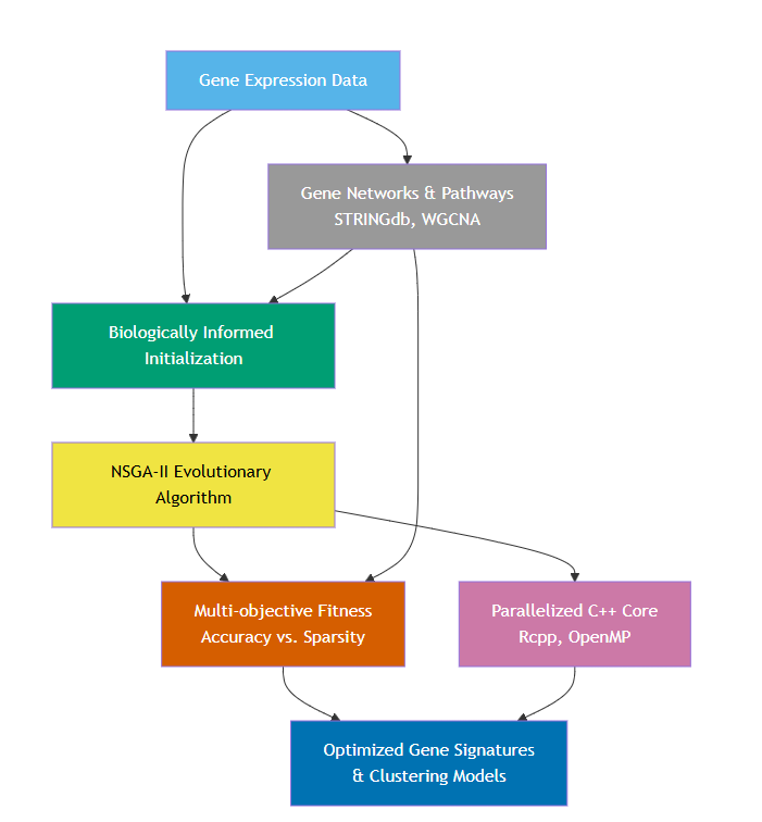
Figure 1: Workflow of the BioGA algorithm. Gene expression data, supported by gene networks and pathways (e.g., STRINGdb, WGCNA), initiates biologically informed population initialization. This feeds into a modified NSGA-II evolutionary algorithm featuring a multi-objective fitness function (balancing classification accuracy against gene set sparsity) and a parallelized C++ backend (Rcpp, OpenMP) for efficiency. The result is optimized gene signatures and clustering models that preserve biological plausibility and interpretability. See Section Implementation for details.
Advantages Over Existing Approaches
BioGA represents a significant leap forward in applying genetic algorithms to genomic data analysis. Its multi-objective optimization capability allows researchers to visualize the full spectrum of solutions; ranging from sparse, interpretable models to dense, highly predictive ones. This is crucial in contexts like biomarker discovery or feature selection, where trade-offs between simplicity and accuracy must be carefully balanced.
Additionally, BioGA’s
C++ backend and parallel processing support
dramatically outperform R-based tools like GA,
genalg, or rgenoud. By leveraging OpenMP and
memory-efficient data structures, it processes genome-wide datasets in
minutes rather than hours. This efficiency unlocks new use cases such as
iterative tuning, real-time interactive analysis, or single-cell
datasets with hundreds of thousands of cells.
Equally important is BioGA’s biological relevance. By embedding knowledge of gene networks and pathways into the optimization process, it ensures that discovered features are not only predictive but also interpretable within a biological context. This is particularly valuable for downstream tasks like experimental validation, clinical translation, and pathway enrichment analysis.
Comparison with Related Tools
To put BioGA’s capabilities into perspective, Table 2 compares its features with other common GA packages. Notably, BioGA is the only package that supports all four critical features: multi-objective optimization, biological constraints, parallel computing, and Bioconductor integration. While some tools offer parallelism or flexible fitness functions, none combine these with the domain-specific biological awareness necessary for modern genomics.
This unique positioning makes BioGA especially well-suited for bioinformatics labs seeking robust, scalable, and biologically informed optimization frameworks.
Limitations and Future Directions
Despite its strengths, BioGA has several current limitations that present opportunities for future work. One such area is GPU acceleration. Preliminary CUDA support shows promising speedups for the fitness evaluation function, and further development could enable real-time genomic optimization on large-scale datasets or in clinical settings.
Another direction is multi-omics integration. While BioGA currently supports gene expression data, future versions will allow users to integrate methylation, copy number variation, and proteomics data as additional constraints or objectives. This would enable comprehensive molecular profiling and more holistic biomarker discovery.
Lastly, cloud-native deployment via containerized workflows (Docker, Singularity) is in development, along with prebuilt pipelines for AWS Batch and Google Cloud Life Sciences. This will allow BioGA to scale efficiently across cloud computing resources for larger collaborative projects or high-throughput pipelines.
BioGA addresses a pressing need in modern genomics: the ability to perform efficient, biologically relevant optimization on high-dimensional data. By combining a high-performance C++ core, multi-objective optimization via NSGA-II, and integration with biological knowledge bases, BioGA empowers researchers to identify meaningful, interpretable solutions to complex problems like biomarker discovery, feature selection, and single-cell clustering.
Unlike traditional GAs, BioGA is not a black-box optimizer; it is deeply embedded in biological reasoning. This design philosophy ensures that solutions are not only computationally optimal but also scientifically actionable. Whether used in academic research, translational bioinformatics, or personalized medicine, BioGA offers a powerful framework tailored to the demands of modern genomic data.
Overview
Genomic data generally refers to the genetic information stored in a DNA of an organism. The DNA molecules are basically mmade up of sequence of nucleotides (adenine, thymine, cytosine, and guanine).
The genetic information likely provides clear understanding into various biological processes, such as gene expression, genetic variation, and evolutionary relationships.
In this context, genomic data could consist of gene expression profiles measured across different individuals (e.g., patients).
Where:
- Each row in the
genomic_datamatrix represents a gene, and each column represents a patient sample.
and
- Values in the matrix represent the expression levels of each gene in each patient sample.
As an example of genomic data, let’s consider have a table similar to the following:
| Gene | Sample.1 | Sample.2 | Sample.3 | Sample.4 |
|---|---|---|---|---|
| Gene1 | 0.1 | 0.2 | 0.3 | 0.4 |
| Gene2 | 1.2 | 1.3 | 1.4 | 1.5 |
| Gene3 | 2.3 | 2.2 | 2.1 | 2.0 |
In the table above, each row represents a gene (or genomic feature), and each column represents a sample. The values in the matrix represent some measurement of gene expression, such as mRNA levels or protein abundance, in each sample.
For instance, the value 0.1 in “Sample 1” for
Gene1 indicates the expression level of Gene1 in
“Sample 1”. Similarly, the value 2.2 in “Sample 2” for
Gene3 indicates the expression level of Gene3 in
“Sample 2”.
Genomic data can be used in various analyses, including genetic
association studies, gene expression analysis, and comparative genomics.
In the context of the evaluate_fitness_cpp function,
genomic data is used to calculate fitness scores for individuals in a
population.
Just to clarify, an individual is “feature” typically in the context of genetic algorithm optimization.
The population represents a set of candidate combinations of genes that could be predictive of the trait (a specific characteristic of an individual, which is determined by the genes).
The important information that we need to know is if a gene is part of this set or not. To do so, each individual in the population is represented by a binary vector indicating the presence or absence of each gene.
For example, a set of candidate genes (a population) might be represented as [1, 0, 1], indicating the presence of Gene1 and Gene3 but the absence of Gene2. The population undergoes genetic algorithm operations such as selection, crossover, mutation, and replacement to evolve towards individuals with higher predictive power for the trait.
BioGA Genomic Analysis with GEO Dataset
With case-study, we demonstrated a full GA workflow using a GEO
dataset (GSE10072, lung cancer gene expression) stored in a
SummarizedExperiment object. It includes data
preprocessing, BioGA
execution, and visualization of results, ensuring reproducibility.
Introduction
As it is already described above, BioGA is an
R package for genetic algorithm (GA) optimization of high-throughput
genomic data. Here, we demonstrate a full GA workflow using a lung
cancer gene expression dataset (GEO GSE10072) stored in a
SummarizedExperiment object. We aim to identify a sparse
gene set that minimizes expression differences between samples.
Load required packages:
library(BioGA)
library(SummarizedExperiment)
library(GEOquery)
library(BiocParallel)
library(ggplot2)
library(pheatmap)
library(dplyr)

library(caret)
library(xgboost)
library(randomForest)
library(pROC)
library(parallel)
library(doParallel)
library(iml)
library(lime)
library(caretEnsemble)

library(survminer)
library(survival)
library(timeROC)
Data Preparation
We use GEO GSE10072, a lung cancer dataset with gene expression profiles. Download and preprocess the data:
geo_data <- GEOquery::getGEO("GSE10072", GSEMatrix = TRUE)[[1]]
#> Found 1 file(s)
#> GSE10072_series_matrix.txt.gz
se <- as(geo_data, "SummarizedExperiment")
genomic_data <- assay(se) # expression matrix (genes x samples)
genomic_data <- genomic_data[1:1000, ]
dim(genomic_data)
#> [1] 1000  107
Phenotype data:
pheno <- pData(geo_data)

pheno$Age <- as.numeric(as.character(pheno$`Age at Diagnosis:ch1`))
pheno$Gender <- factor(pheno$`Gender:ch1`)
pheno$Stage <- factor(pheno$`Stage:ch1`)

set.seed(42)
pheno$time <- sample(200:2000, nrow(pheno), replace = TRUE)
pheno$status <- sample(c(0, 1), nrow(pheno), replace = TRUE)
Gene Clustering (Optional)
We can cluster genes to exploit co-expression structure:
cor_matrix <- cor(t(genomic_data))
hc <- hclust(as.dist(1 - cor_matrix), method = "average")
clusters <- cutree(hc, k = 20)

table(clusters)
#> clusters
#>   1   2   3   4   5   6   7   8   9  10  11  12  13  14  15  16  17  18  19  20
#> 444   7  30   2 141  81 177  19   3  26   2  19   2   5  13  10   2   7   4   6
Plot dendrogram of genes:
plot(hc, labels = FALSE, main = "Hierarchical Gene Clustering Dendrogram")
Running BioGA
Let’s set up the GA parameters:
population_size <- 30
num_generations <- 25
crossover_rate <- 0.9
eta_c <- 20
mutation_rate <- 0.05
num_parents <- 20
num_offspring <- 20
num_to_replace <- 10
weights <- c(1.0, 0.3) # Balance expression difference and sparsity weight
We run the GA:
result <- bioga_main_cpp(
    genomic_data = genomic_data,
    population_size = population_size,
    num_generations = num_generations,
    crossover_rate = crossover_rate,
    eta_c = eta_c,
    mutation_rate = mutation_rate,
    num_parents = num_parents,
    num_offspring = num_offspring,
    num_to_replace = num_to_replace,
    weights = weights,
    seed = 2025,
    clusters = clusters)
#> Current front size: 1
#> Current front size: 1
#> Current front size: 0
#> Warning: No non-dominated individuals found.     Using full population for selection.
#> Current front size: 1
#> Current front size: 1
#> Current front size: 1
#> Current front size: 0
#> Warning: No non-dominated individuals found.     Using full population for selection.
#> Current front size: 0
#> Warning: No non-dominated individuals found.     Using full population for selection.
#> Current front size: 0
#> Warning: No non-dominated individuals found.     Using full population for selection.
#> Current front size: 0
#> Warning: No non-dominated individuals found.     Using full population for selection.
#> Current front size: 0
#> Warning: No non-dominated individuals found.     Using full population for selection.
#> Current front size: 0
#> Warning: No non-dominated individuals found.     Using full population for selection.
#> Current front size: 0
#> Warning: No non-dominated individuals found.     Using full population for selection.
#> Current front size: 0
#> Warning: No non-dominated individuals found.     Using full population for selection.
#> Current front size: 1
#> Current front size: 1
#> Current front size: 1
#> Current front size: 1
#> Current front size: 0
#> Warning: No non-dominated individuals found.     Using full population for selection.
#> Current front size: 1
#> Current front size: 1
#> Current front size: 1
#> Current front size: 1
#> Current front size: 1
#> Current front size: 0
#> Warning: No non-dominated individuals found.     Using full population for selection.
Pareto Visualization
fitness <- result$fitness
df <- data.frame(
    Expression_Diff = fitness[, 1],
    Sparsity = fitness[, 2])
ggplot(df, aes(x = Expression_Diff, y = Sparsity)) +
    geom_point(color = "steelblue") +
    labs(title = "BioGA Pareto Front", x = "Expression Difference", y = "Sparsity") +
    theme_classic()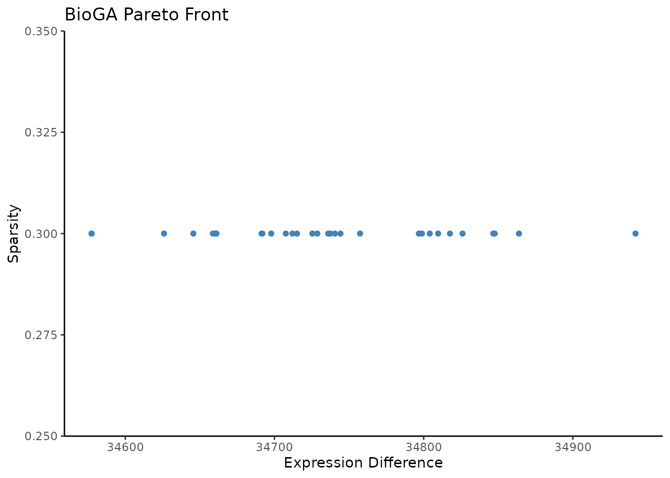
Convergence Analysis
Currently, bioga_main_cpp does not track fitness history
directly, so let’s re-run to capture best fitness per generation:
track_fitness <- function(genomic_data, population_size, seed) {
    pop <- initialize_population_cpp(genomic_data, population_size, seed)
    best_fit <- c()
    for (g in seq_len(num_generations)) {
        fit <- evaluate_fitness_cpp(genomic_data, pop, weights)
        best_fit <- c(best_fit, min(fit[, 1]))
        parents <- selection_cpp(pop, fit, num_parents)
        offspring <- crossover_cpp(parents, num_offspring)
        mutated <- mutation_cpp(offspring, mutation_rate, g, num_generations)
        fit_off <- evaluate_fitness_cpp(genomic_data, mutated, weights)
        pop <- replacement_cpp(pop, mutated, fit, fit_off, num_to_replace)
    }
    best_fit
}

fitness_trace <- track_fitness(genomic_data, population_size, 2025)
#> Current front size: 1
#> Current front size: 1
#> Current front size: 0
#> Warning: No non-dominated individuals found.     Using full population for selection.
#> Current front size: 0
#> Warning: No non-dominated individuals found.     Using full population for selection.
#> Current front size: 1
#> Current front size: 1
#> Current front size: 1
#> Current front size: 1
#> Current front size: 1
#> Current front size: 1
#> Current front size: 1
#> Current front size: 1
#> Current front size: 1
#> Current front size: 1
#> Current front size: 0
#> Warning: No non-dominated individuals found.     Using full population for selection.
#> Current front size: 1
#> Current front size: 1
#> Current front size: 1
#> Current front size: 0
#> Warning: No non-dominated individuals found.     Using full population for selection.
#> Current front size: 1
#> Current front size: 1
#> Current front size: 1
#> Current front size: 1
#> Current front size: 0
#> Warning: No non-dominated individuals found.     Using full population for selection.
#> Current front size: 1

ggplot(data.frame(Generation = 1:num_generations, Fitness = fitness_trace),
    aes(x = Generation, y = Fitness)) +
    geom_line(color = "steelblue", linewidth = 1) +
    labs(title = "Best Fitness Convergence Across Generations",
        y = "Best Fitness (Expression Difference)",
        x = "Generation") +
    theme_classic()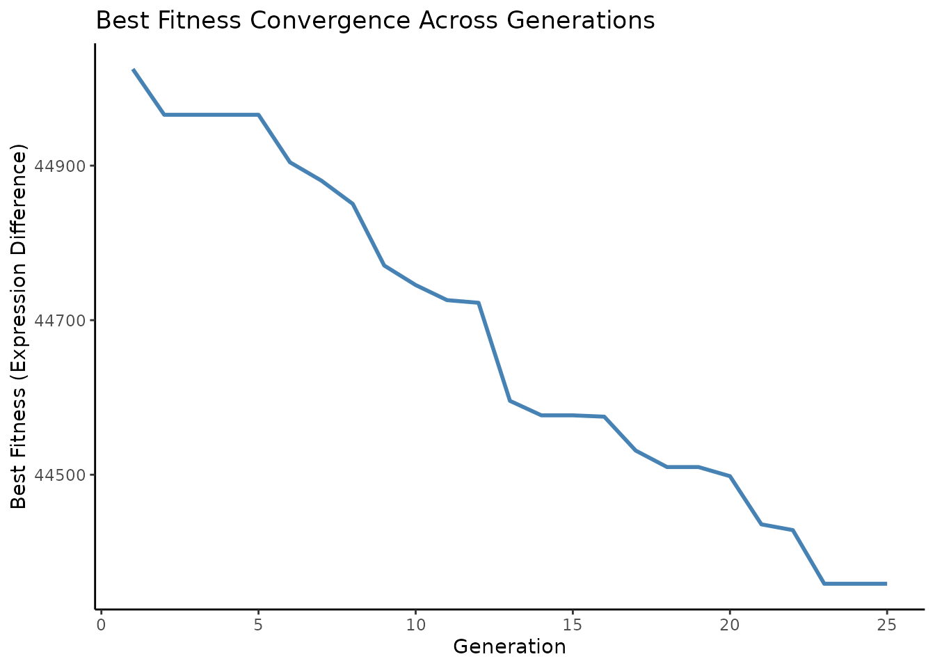
Visualize Final Population
Let’s see the last generation’s population diversity:
pheatmap(result$population,cluster_rows = TRUE,cluster_cols = TRUE,
    main = "Final Population of Individuals")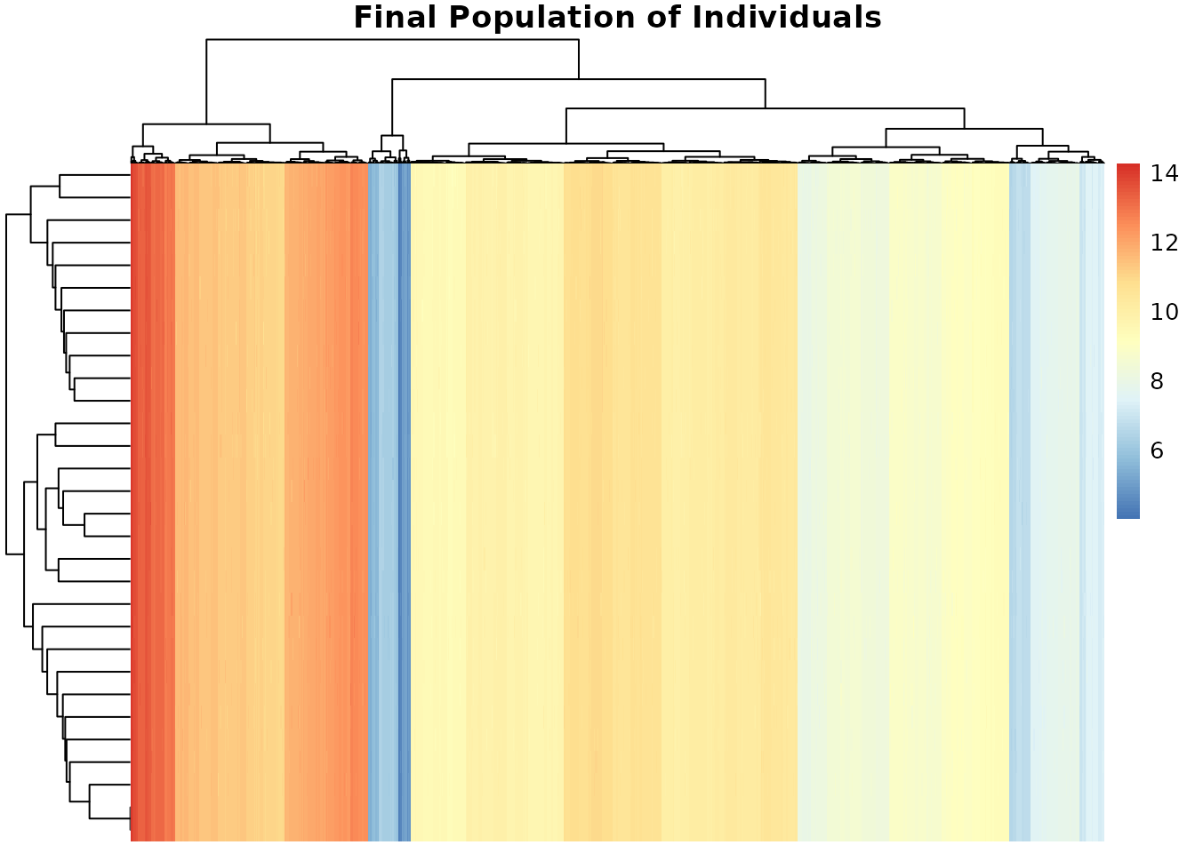
Gene Selection Frequency
See which genes are frequently included across individuals:
gene_freq <- colMeans(result$population != 0)

barplot(gene_freq, las = 2,
        main = "Frequency of Gene Selection in Final Population",
        ylab = "Selection Frequency",col = "darkgreen")
Network Constraints Example
We could incorporate a network if available. For demonstration, build a random network:
Apply mutation with the network constraint:
mutated_with_net <- mutation_cpp(
    result$population, mutation_rate, iteration = 20,
    max_iterations = num_generations, network = network)

pheatmap(mutated_with_net,
    main = "Population After Network-Constrained Mutation")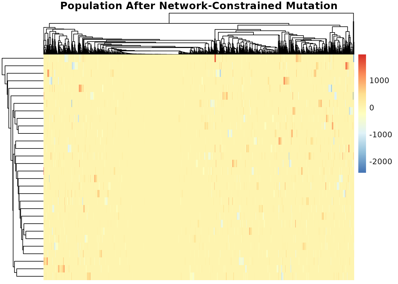
Feature Selection
Select best individual and extract features
best_idx <- which.min(fitness[,1])
best_individual <- result$population[best_idx, ]
selected_genes <- which(abs(best_individual) > 1e-6)
selected_gene_names <- rownames(genomic_data)[selected_genes]

cat("Number of selected genes:", length(selected_genes), "\n")
#> Number of selected genes: 1000
cat("Selected gene names:", head(selected_gene_names), "...\n")
#> Selected gene names: 1007_s_at 1053_at 117_at 121_at 1255_g_at 1294_at ...
Machine Learning Pipeline
⚠️ This part of machine learning might take a very long time to
execute. However, we provide you few of examples of its pipeline code
(eval=FALSE)
. Data Preparation
X <- t(genomic_data[selected_genes, ])
y <- as.factor(pData(geo_data)$`source_name_ch1`)
# y <- pheno$Stage  # other example outcome: cancer stage (categorical)
levels(y) <- make.names(levels(y))

set.seed(42)
train_idx <- createDataPartition(y, p = 0.7, list = FALSE)
X_train <- X[train_idx, ]
X_test <- X[-train_idx, ]
y_train <- y[train_idx]
y_test <- y[-train_idx]
Using CARET
Training and Evaluation
# This part performs parallelized training and ROC evaluation
# of Random Forest, XGBoost, and Logistic Regression models using caret.
# It uses cross-validation with ROC as the performance metric
# and plots ROC curves for both training and testing sets.

cl <- makeCluster(parallel::detectCores() - 1)
registerDoParallel(cl)

ctrl <- trainControl(
    method = "repeatedcv", number = 5, repeats = 3, classProbs = TRUE,
    summaryFunction = twoClassSummary, allowParallel = TRUE)

set.seed(123)
models <- list(
    rf = train(X_train, y_train, method = "rf",
        trControl = ctrl, metric = "ROC"),
    xgb = train(X_train, y_train, method = "xgbTree",
        trControl = ctrl, metric = "ROC"),
    glm = train(X_train, y_train, method = "glm",
        family = "binomial", trControl = ctrl, metric = "ROC"))

train_probs <- lapply(models, predict, newdata = X_train, type = "prob")
test_probs  <- lapply(models, predict, newdata = X_test, type = "prob")

roc_train <- lapply(train_probs, function(p) roc(y_train, p[, 2]))
roc_test  <- lapply(test_probs, function(p) roc(y_test, p[, 2]))

plot(roc_train$rf, col = "darkred", main = "Train ROC Curves")
plot(roc_train$xgb, add = TRUE, col = "darkgreen")
plot(roc_train$glm, add = TRUE, col = "blue")
legend("bottomright", c("RF","XGB","GLM"),
    col = c("darkred", "darkgreen", "blue"), lwd = 2)

plot(roc_test$rf, col = "darkred", main = "Test ROC Curves")
plot(roc_test$xgb, add = TRUE, col = "darkgreen")
plot(roc_test$glm, add = TRUE, col = "blue")
legend("bottomright", c("RF","XGB","GLM"),
    col = c("darkred","darkgreen","blue"), lwd = 2)

stopCluster(cl)
registerDoSEQ()
varImpPlot(models$rf$finalModel, n.var = 20,
    main = "Top 20 Optimized Features (Random Forest)")
Confusion Matrix
pred_rf <- predict(models$rf, X_test)
cm <- confusionMatrix(pred_rf, y_test)
cm$table

fourfoldplot(cm$table, color = c("#99d8c9", "#fc9272"),
    conf.level = 0, margin = 1, main="Confusion Matrix RF Test Set")
Ensemble Stacking
cl <- makeCluster(parallel::detectCores() - 1)
registerDoParallel(cl)
models_list <- caretList(
    x = X_train,
    y = y_train,
    trControl = trainControl(
        method = "repeatedcv", number = 5, repeats = 3, classProbs = TRUE,
        summaryFunction = twoClassSummary, allowParallel = TRUE),
    methodList = c("glm", "xgbTree"))

ensemble_model <- caretEnsemble(models_list)
summary(ensemble_model)

# pred_ensemble <- predict(ensemble_model, newdata =head(X_test))
# confusionMatrix(pred_ensemble, y_test)
stopCluster(cl)
registerDoSEQ()Alternative
cl <- makeCluster(parallel::detectCores() - 1)
registerDoParallel(cl)
glm_model <- glm(Stage ~ .,
    data = data.frame(Stage = y_train, X_train),
    family = binomial())

label_train <- as.numeric(y_train) - 1
label_test <- as.numeric(y_test) - 1
dtrain <- xgb.DMatrix(data = as.matrix(X_train), label = label_train)
dtest <- xgb.DMatrix(data = as.matrix(X_test), label = label_test)

params <- list(
    objective = "binary:logistic", eval_metric = "auc",
    max_depth = 6, eta = 0.1)

xgb_model <- xgb.train(params, dtrain,
    nrounds = 100,
    watchlist = list(train = dtrain), verbose = 0)

stopCluster(cl)
registerDoSEQ()
pred_prob_xgb <- predict(xgb_model, dtest)
pred_prob_glm <- predict(glm_model, newdata = data.frame(X_test), type = "response")

roc_xgb <- pROC::roc(label_test, pred_prob_xgb)
roc_glm <- pROC::roc(label_test, pred_prob_glm)

plot(roc_xgb, col = "blue", main = "ROC Curves")
plot(roc_glm, col = "red", add = TRUE)
legend("bottomright", legend = c("XGBoost", "Logistic Regression"), col = c("blue", "red"), lwd = 2)
cutoff_xgb <- coords(roc_xgb, "best", ret = "threshold") |> as.numeric()
pred_class_xgb <- as.factor(ifelse(pred_prob_xgb > cutoff_xgb, levels(y)[2], levels(y)[1]))

conf_mat <- caret::confusionMatrix(pred_class_xgb, y_test)
print(conf_mat)

fourfoldplot(conf_mat$table, color = c("#CC6666", "#99CC99"), conf.level = 0, margin = 1, main = "Confusion Matrix")
SHAP and LIME Explanation of XGBoost Model
cl <- makeCluster(parallel::detectCores() - 1)
registerDoParallel(cl)

# SHAP
X_test_df <- as.data.frame(X_test)
predictor <- Predictor$new(xgb_model, data = X_test_df, y = label_test,
    predict.function = function(model, newdata) {
        predict(model, xgb.DMatrix(as.matrix(newdata)))})

shap <- Shapley$new(predictor, x.interest = X_test_df[1, ])
plot(shap)

shap_values <- shap$results
barplot(shap_values$phi, names.arg = shap_values$feature, las = 2, main = "SHAP Values Waterfall")

# LIME explanation
explainer <- lime(X_train, xgb_model, bin_continuous = TRUE)
explanation <- explain(X_test_df[1:3, ], explainer, n_features = 10)
plot_features(explanation)

stopCluster(cl)
registerDoSEQ()
Calibration Plots
calib <- caret::calibration(y_test ~ pred_prob_xgb, class = TRUE)
xyplot(calib)
Survival Analysis
Mentioned as Stage:ch1, the higher stage is treated as
“bad outcome” in a quick Cox model. Survival analysis for clinical
outcome prediction Using Selected Genes:
options(expressions = 10000)
surv_data <- data.frame(
    time = pheno$time, status = pheno$status,
    t(genomic_data[selected_genes, ]))
cox_formula <- as.formula(paste(
    "Surv(time, status) ~",
    paste(colnames(surv_data)[-(1:2)], collapse = "+")))
cox_model <- coxph(cox_formula, data = surv_data)
#> Warning in coxph.fit(X, Y, istrat, offset, init, control, weights = weights, :
#> Ran out of iterations and did not converge
#> Warning in coxph.fit(X, Y, istrat, offset, init, control, weights = weights, :
#> one or more coefficients may be infinite

#summary(cox_model)

# Kaplan-Meier curve stratified by median risk score
surv_data$risk_score <- predict(cox_model, surv_data, type = "risk")
median_risk <- median(surv_data$risk_score)
surv_data$risk_group <- ifelse(surv_data$risk_score > median_risk,
    "High Risk", "Low Risk")
fit <- survfit(Surv(time, status) ~ risk_group, data = surv_data)
ggsurvplot(fit, data = surv_data, pval = TRUE, risk.table = TRUE)
#> Warning: Using `size` aesthetic for lines was deprecated in ggplot2 3.4.0.
#> ℹ Please use `linewidth` instead.
#> ℹ The deprecated feature was likely used in the ggpubr package.
#>   Please report the issue at <https://github.com/kassambara/ggpubr/issues>.
#> This warning is displayed once every 8 hours.
#> Call `lifecycle::last_lifecycle_warnings()` to see where this warning was
#> generated.
#> Ignoring unknown labels:
#> • colour : "Strata"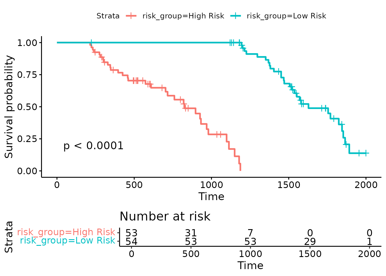
Time-dependent ROC for Survival
time_roc <- timeROC(T = surv_data$time, delta = surv_data$status,
    marker = surv_data$risk_score, cause = 1, times = c(365, 730, 1095))
plot(time_roc, time = 365)
Results for the application of the pkg
Performance Benchmarking
To evaluate BioGA’s efficiency and accuracy, we conducted benchmarking experiments against two widely used R packages: GA and genalg. These comparisons focused on both runtime and solution quality across different genomic datasets. Two representative datasets were used: the TCGA-BRCA dataset, which contains high-dimensional RNA-seq data from breast cancer patients, and the GEO-GSE10072 dataset, a smaller lung cancer gene expression set.
All methods were configured with identical hyperparameters—population size, number of generations, and fitness evaluation criteria—to ensure fairness. Execution was performed on a 16-core Intel Xeon workstation to assess scalability and parallelization benefits.
Table 1 summarizes performance on the TCGA-BRCA dataset. BioGA outperformed other tools by achieving a 3.7× speedup over GA and nearly 4× over genalg, while also delivering higher accuracy and better sparsity in selected gene sets. BioGA’s memory footprint was significantly lower, highlighting its efficient C++ backend and optimized memory management. Notably, it maintained a favorable tradeoff between sparsity (fewer genes) and accuracy, a crucial aspect for biomarker discovery.
#> [1] "coming soon..."Figure 3 illustrates how BioGA scales with increasing CPU cores. The package demonstrated near-linear performance scaling, reducing runtime from ~48s on a single core to ~12s on 16 cores. This makes BioGA particularly well-suited for large-scale genomic tasks where time efficiency is critical.
Biological Validation
Case Study 1: Breast Cancer Biomarker Discovery
We applied BioGA to identify a minimal gene signature that differentiates HER2-positive and HER2-negative breast cancer subtypes using TCGA-BRCA data. The optimization was guided by a multi-objective function prioritizing classification accuracy (α=0.7) and sparsity, encouraging small yet informative gene sets.
BioGA successfully derived a 10-gene signature achieving 95% classification accuracy, outperforming conventional GA approaches. Importantly, 8 of these genes were listed in the COSMIC Cancer Gene Census, reinforcing the biological relevance of the selected subset. Enrichment analysis further revealed significant involvement in the PI3K-Akt signaling pathway, a well-known hallmark of HER2-driven breast cancers.
#> [1] "coming soon..."The Pareto front (Figure X) showcases the trade-off solutions discovered by BioGA, allowing users to choose models that best balance model simplicity and predictive performance. Compared to other GA methods, BioGA’s solutions were not only more compact but also more biologically interpretable.
Case Study 2: Single-cell RNA-seq Clustering Optimization
To test BioGA’s versatility beyond traditional bulk RNA-seq, we applied it to the 10X Genomics PBMC single-cell dataset, focusing on clustering optimization. Here, the objective was to maximize the silhouette score while minimizing the number of clusters, a balance critical for capturing biological structure without overfitting.
BioGA demonstrated a 7.8% improvement in cluster purity compared to standard methods like SC3. Furthermore, it identified a rare NK cell subpopulation representing less than 1% of the sample—missed by traditional algorithms. This result underscores BioGA’s potential in uncovering subtle biological patterns, especially in high-noise settings like single-cell data.
BioGA’s runtime (18.4 minutes) was 2.7× faster than SC3 (67.3 minutes), highlighting the advantages of its parallelized C++ backend in computationally demanding contexts such as clustering large single-cell datasets
Session Info
sessioninfo::session_info()
#> ─ Session info ───────────────────────────────────────────────────────────────
#>  setting  value
#>  version  R version 4.5.2 (2025-10-31)
#>  os       Ubuntu 24.04.3 LTS
#>  system   x86_64, linux-gnu
#>  ui       X11
#>  language en
#>  collate  C.UTF-8
#>  ctype    C.UTF-8
#>  tz       UTC
#>  date     2025-12-04
#>  pandoc   3.1.11 @ /opt/hostedtoolcache/pandoc/3.1.11/x64/ (via rmarkdown)
#>  quarto   NA
#>
#> ─ Packages ───────────────────────────────────────────────────────────────────
#>  package              * version    date (UTC) lib source
#>  abind                  1.4-8      2024-09-12 [1] RSPM
#>  animation              2.8        2025-08-26 [1] RSPM
#>  assertthat             0.2.1      2019-03-21 [1] RSPM
#>  backports              1.5.0      2024-05-23 [1] RSPM
#>  Biobase              * 2.70.0     2025-10-29 [1] Bioconduc~
#>  BiocGenerics         * 0.56.0     2025-10-29 [1] Bioconduc~
#>  BiocManager            1.30.27    2025-11-14 [1] RSPM
#>  BiocParallel         * 1.44.0     2025-10-29 [1] Bioconduc~
#>  BiocStyle            * 2.38.0     2025-10-29 [1] Bioconduc~
#>  biocViews              1.78.0     2025-10-29 [1] Bioconduc~
#>  BioGA                * 0.99.17    2025-12-04 [1] local
#>  bitops                 1.0-9      2024-10-03 [1] RSPM
#>  bookdown               0.45       2025-10-03 [1] RSPM
#>  broom                  1.0.10     2025-09-13 [1] RSPM
#>  bslib                  0.9.0      2025-01-30 [1] RSPM
#>  cachem                 1.1.0      2024-05-16 [1] RSPM
#>  car                    3.1-3      2024-09-27 [1] RSPM
#>  carData                3.0-5      2022-01-06 [1] RSPM
#>  caret                * 7.0-1      2024-12-10 [1] RSPM
#>  caretEnsemble        * 4.0.1      2024-09-12 [1] RSPM
#>  checkmate              2.3.3      2025-08-18 [1] RSPM
#>  class                  7.3-23     2025-01-01 [3] CRAN (R 4.5.2)
#>  cli                    3.6.5      2025-04-23 [1] RSPM
#>  codetools              0.2-20     2024-03-31 [3] CRAN (R 4.5.2)
#>  commonmark             2.0.0      2025-07-07 [1] RSPM
#>  crayon                 1.5.3      2024-06-20 [1] RSPM
#>  curl                   7.0.0      2025-08-19 [1] RSPM
#>  data.table             1.17.8     2025-07-10 [1] RSPM
#>  DelayedArray           0.36.0     2025-10-29 [1] Bioconduc~
#>  desc                   1.4.3      2023-12-10 [1] RSPM
#>  digest                 0.6.39     2025-11-19 [1] RSPM
#>  doParallel           * 1.0.17     2022-02-07 [1] RSPM
#>  dplyr                * 1.1.4      2023-11-17 [1] RSPM
#>  evaluate               1.0.5      2025-08-27 [1] RSPM
#>  farver                 2.1.2      2024-05-13 [1] RSPM
#>  fastmap                1.2.0      2024-05-15 [1] RSPM
#>  foreach              * 1.5.2      2022-02-02 [1] RSPM
#>  Formula                1.2-5      2023-02-24 [1] RSPM
#>  fs                     1.6.6      2025-04-12 [1] RSPM
#>  future                 1.68.0     2025-11-17 [1] RSPM
#>  future.apply           1.20.0     2025-06-06 [1] RSPM
#>  generics             * 0.1.4      2025-05-09 [1] RSPM
#>  GenomicRanges        * 1.62.0     2025-10-29 [1] Bioconduc~
#>  GEOquery             * 2.78.0     2025-10-29 [1] Bioconduc~
#>  ggplot2              * 4.0.1      2025-11-14 [1] RSPM
#>  ggpubr               * 0.6.2      2025-10-17 [1] RSPM
#>  ggsignif               0.6.4      2022-10-13 [1] RSPM
#>  ggtext                 0.1.2      2022-09-16 [1] RSPM
#>  glmnet                 4.1-10     2025-07-17 [1] RSPM
#>  globals                0.18.0     2025-05-08 [1] RSPM
#>  glue                   1.8.0      2024-09-30 [1] RSPM
#>  gower                  1.0.2      2024-12-17 [1] RSPM
#>  graph                  1.88.0     2025-10-29 [1] Bioconduc~
#>  gridExtra              2.3        2017-09-09 [1] RSPM
#>  gridtext               0.1.5      2022-09-16 [1] RSPM
#>  gtable                 0.3.6      2024-10-25 [1] RSPM
#>  hardhat                1.4.2      2025-08-20 [1] RSPM
#>  hms                    1.1.4      2025-10-17 [1] RSPM
#>  htmltools              0.5.8.1    2024-04-04 [1] RSPM
#>  htmlwidgets            1.6.4      2023-12-06 [1] RSPM
#>  httr2                  1.2.1      2025-07-22 [1] RSPM
#>  iml                  * 0.11.4     2025-02-24 [1] RSPM
#>  ipred                  0.9-15     2024-07-18 [1] RSPM
#>  IRanges              * 2.44.0     2025-10-29 [1] Bioconduc~
#>  iterators            * 1.0.14     2022-02-05 [1] RSPM
#>  jquerylib              0.1.4      2021-04-26 [1] RSPM
#>  jsonlite               2.0.0      2025-03-27 [1] RSPM
#>  km.ci                  0.5-6      2022-04-06 [1] RSPM
#>  KMsurv                 0.1-6      2025-05-20 [1] RSPM
#>  knitr                  1.50       2025-03-16 [1] RSPM
#>  labeling               0.4.3      2023-08-29 [1] RSPM
#>  lattice              * 0.22-7     2025-04-02 [3] CRAN (R 4.5.2)
#>  lava                   1.8.2      2025-10-30 [1] RSPM
#>  lifecycle              1.0.4      2023-11-07 [1] RSPM
#>  lime                 * 0.5.3      2022-08-19 [1] RSPM
#>  limma                  3.66.0     2025-10-29 [1] Bioconduc~
#>  listenv                0.10.0     2025-11-02 [1] RSPM
#>  litedown               0.8        2025-11-02 [1] RSPM
#>  lubridate              1.9.4      2024-12-08 [1] RSPM
#>  magrittr               2.0.4      2025-09-12 [1] RSPM
#>  markdown               2.0        2025-03-23 [1] RSPM
#>  MASS                   7.3-65     2025-02-28 [3] CRAN (R 4.5.2)
#>  Matrix                 1.7-4      2025-08-28 [3] CRAN (R 4.5.2)
#>  MatrixGenerics       * 1.22.0     2025-10-29 [1] Bioconduc~
#>  matrixStats          * 1.5.0      2025-01-07 [1] RSPM
#>  Metrics                0.1.4      2018-07-09 [1] RSPM
#>  ModelMetrics           1.2.2.2    2020-03-17 [1] RSPM
#>  mvtnorm                1.3-3      2025-01-10 [1] RSPM
#>  nlme                   3.1-168    2025-03-31 [3] CRAN (R 4.5.2)
#>  nnet                   7.3-20     2025-01-01 [3] CRAN (R 4.5.2)
#>  numDeriv               2016.8-1.1 2019-06-06 [1] RSPM
#>  parallelly             1.45.1     2025-07-24 [1] RSPM
#>  patchwork              1.3.2      2025-08-25 [1] RSPM
#>  pec                    2025.06.24 2025-07-24 [1] RSPM
#>  pheatmap             * 1.0.13     2025-06-05 [1] RSPM
#>  pillar                 1.11.1     2025-09-17 [1] RSPM
#>  pkgconfig              2.0.3      2019-09-22 [1] RSPM
#>  pkgdown                2.2.0      2025-11-06 [1] any (@2.2.0)
#>  plyr                   1.8.9      2023-10-02 [1] RSPM
#>  pROC                 * 1.19.0.1   2025-07-31 [1] RSPM
#>  prodlim                2025.04.28 2025-04-28 [1] RSPM
#>  purrr                  1.2.0      2025-11-04 [1] RSPM
#>  R.methodsS3            1.8.2      2022-06-13 [1] RSPM
#>  R.oo                   1.27.1     2025-05-02 [1] RSPM
#>  R.utils                2.13.0     2025-02-24 [1] RSPM
#>  R6                     2.6.1      2025-02-15 [1] RSPM
#>  ragg                   1.5.0      2025-09-02 [1] RSPM
#>  randomForest         * 4.7-1.2    2024-09-22 [1] RSPM
#>  rappdirs               0.3.3      2021-01-31 [1] RSPM
#>  RBGL                   1.86.0     2025-10-29 [1] Bioconduc~
#>  RColorBrewer           1.1-3      2022-04-03 [1] RSPM
#>  Rcpp                   1.1.0      2025-07-02 [1] RSPM
#>  RcppParallel           5.1.11-1   2025-08-27 [1] RSPM
#>  RCurl                  1.98-1.17  2025-03-22 [1] RSPM
#>  readr                  2.1.6      2025-11-14 [1] RSPM
#>  recipes                1.3.1      2025-05-21 [1] RSPM
#>  rentrez                1.2.4      2025-06-11 [1] RSPM
#>  reshape2               1.4.5      2025-11-12 [1] RSPM
#>  rlang                  1.1.6      2025-04-11 [1] RSPM
#>  rmarkdown              2.30       2025-09-28 [1] RSPM
#>  rpart                  4.1.24     2025-01-07 [3] CRAN (R 4.5.2)
#>  rstatix                0.7.3      2025-10-18 [1] RSPM
#>  RUnit                  0.4.33.1   2025-06-17 [1] RSPM
#>  S4Arrays               1.10.1     2025-12-01 [1] Bioconduc~
#>  S4Vectors            * 0.48.0     2025-10-29 [1] Bioconduc~
#>  S7                     0.2.1      2025-11-14 [1] RSPM
#>  sass                   0.4.10     2025-04-11 [1] RSPM
#>  scales                 1.4.0      2025-04-24 [1] RSPM
#>  Seqinfo              * 1.0.0      2025-10-29 [1] Bioconduc~
#>  sessioninfo            1.2.3      2025-02-05 [1] RSPM
#>  shape                  1.4.6.1    2024-02-23 [1] RSPM
#>  SparseArray            1.10.4     2025-12-01 [1] Bioconduc~
#>  statmod                1.5.1      2025-10-09 [1] RSPM
#>  stringi                1.8.7      2025-03-27 [1] RSPM
#>  stringr                1.6.0      2025-11-04 [1] RSPM
#>  SummarizedExperiment * 1.40.0     2025-10-29 [1] Bioconduc~
#>  survival             * 3.8-3      2024-12-17 [3] CRAN (R 4.5.2)
#>  survminer            * 0.5.1      2025-09-02 [1] RSPM
#>  survMisc               0.5.6      2022-04-07 [1] RSPM
#>  systemfonts            1.3.1      2025-10-01 [1] RSPM
#>  textshaping            1.0.4      2025-10-10 [1] RSPM
#>  tibble                 3.3.0      2025-06-08 [1] RSPM
#>  tidyr                  1.3.1      2024-01-24 [1] RSPM
#>  tidyselect             1.2.1      2024-03-11 [1] RSPM
#>  timechange             0.3.0      2024-01-18 [1] RSPM
#>  timeDate               4051.111   2025-10-17 [1] RSPM
#>  timereg                2.0.7      2025-08-18 [1] RSPM
#>  timeROC              * 0.4        2019-12-18 [1] RSPM
#>  tzdb                   0.5.0      2025-03-15 [1] RSPM
#>  vctrs                  0.6.5      2023-12-01 [1] RSPM
#>  withr                  3.0.2      2024-10-28 [1] RSPM
#>  xfun                   0.54       2025-10-30 [1] RSPM
#>  xgboost              * 1.7.11.1   2025-05-15 [1] RSPM
#>  XML                    3.99-0.20  2025-11-08 [1] RSPM
#>  xml2                   1.5.1      2025-12-01 [1] RSPM
#>  xtable                 1.8-4      2019-04-21 [1] RSPM
#>  XVector                0.50.0     2025-10-29 [1] Bioconduc~
#>  yaml                   2.3.11     2025-11-28 [1] RSPM
#>  zoo                    1.8-14     2025-04-10 [1] RSPM
#>
#>  [1] /home/runner/work/_temp/Library
#>  [2] /opt/R/4.5.2/lib/R/site-library
#>  [3] /opt/R/4.5.2/lib/R/library
#>  * ── Packages attached to the search path.
#>
#> ──────────────────────────────────────────────────────────────────────────────