Usage Demonstration of BioGA
Multi-Objective Genetic Algorithm for Genomic Data Analysis
Dany Mukesha
2025-12-04
Source:vignettes/UsageDemostration.Rmd
UsageDemostration.RmdIntroduction to BioGA
BioGA is a powerful R package designed to execute a
multi-objective Genetic Algorithm (GA) tailored for the optimization of
high-dimensional genomic data. This approach is highly effective in
scenarios where multiple, often conflicting, biological and statistical
objectives must be satisfied simultaneously.
This vignette provides a hands-on guide, walking through the essential steps of preparing data, running the GA, and interpreting the critical results, including convergence, diversity, and gene selection frequency.
1. Prepare Simulated Genomic Data
We begin by simulating a typical gene expression matrix, mimicking data from a microarray or RNA-sequencing experiment. The data will feature two classes (Control and Case) and will include a subset of differentially expressed genes to provide a clear optimization target.
set.seed(123)
n_genes <- 50
n_samples <- 20

# Simulate base expression data (50 genes x 20 samples)
genomic_data <- matrix(rnorm(n_genes * n_samples, mean = 5, sd = 2),
    nrow = n_genes, ncol = n_samples)

# Define class labels and introduce differential expression for the first 10 genes
class_labels <- rep(c("Control", "Case"), each = 10)
DE_genes_indices <- 1:10
genomic_data[DE_genes_indices, class_labels == "Case"] <-
    genomic_data[DE_genes_indices, class_labels == "Case"] + 3

rownames(genomic_data) <- paste0("Gene", 1:n_genes)
colnames(genomic_data) <- paste0("Sample", 1:n_samples)

# Create annotation bar for visualization
col_annotation <- data.frame(Class = factor(class_labels))
rownames(col_annotation) <- colnames(genomic_data)
Data Visualization (Heatmap)
A heatmap visually confirms the structure of the simulated data, allowing us to see the clusters formed by the differentially expressed genes and the samples.
pheatmap(genomic_data,
    cluster_rows = TRUE, cluster_cols = TRUE,
    annotation_col = col_annotation,
    main = "Simulated Gene Expression Data Structure",
    show_colnames = FALSE)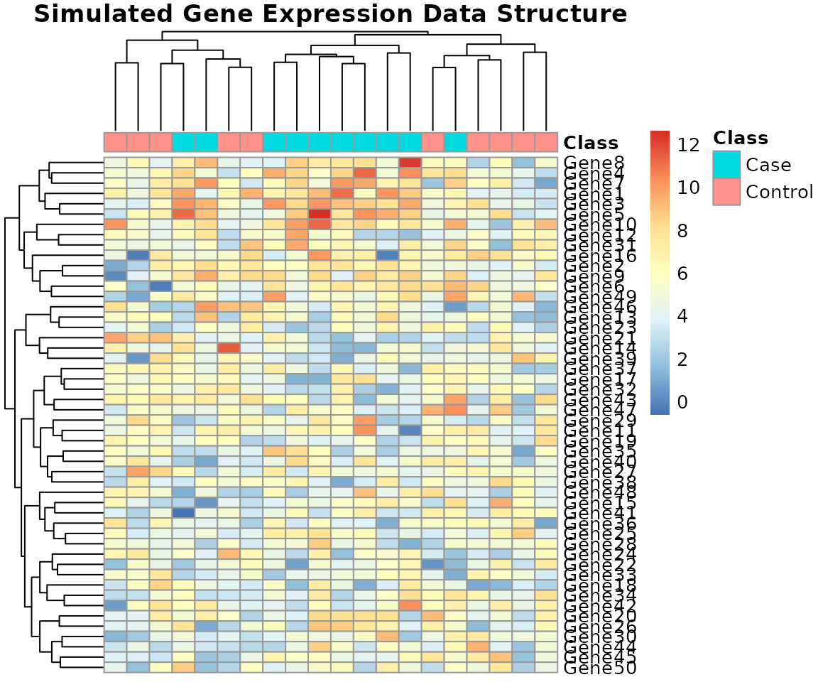
2. Run the Genetic Algorithm
The core of the analysis involves running the multi-objective GA
using the bioga_main_cpp function. We specify key
parameters defining the evolutionary process and the objectives.
GA Parameters
The GA is configured using standard parameters common to evolutionary computation:
| Parameter | Value | Description |
|---|---|---|
population_size |
30 | Number of individuals in the population. |
num_generations |
50 | Total number of evolutionary steps. |
crossover_rate |
0.9 | Probability of performing Crossover (SBX). |
eta_c |
20.0 | Distribution index for SBX (controls locality). |
mutation_rate |
0.1 | Base probability of mutation. |
weights |
c(1.0, 0.5) |
Weights for (, ). (Expression Difference) is prioritized over (Sparsity). |
result <- bioga_main_cpp(
    genomic_data = genomic_data,
    population_size = 30,
    num_generations = 50,
    crossover_rate = 0.9,
    eta_c = 20.0,
    mutation_rate = 0.1,
    num_parents = 20,
    num_offspring = 20,
    num_to_replace = 10,
    weights = c(1.0, 0.5), # w1*f1 + w2*f2
    seed = 42
)
#> Current front size: 1
#> Current front size: 1
#> Current front size: 1
#> Current front size: 1
#> Current front size: 1
#> Current front size: 1
#> Current front size: 1
#> Current front size: 1
#> Current front size: 1
#> Current front size: 1
#> Current front size: 1
#> Current front size: 1
#> Current front size: 1
#> Current front size: 1
#> Current front size: 1
#> Current front size: 1
#> Current front size: 1
#> Current front size: 1
#> Current front size: 1
#> Current front size: 1
#> Current front size: 1
#> Current front size: 1
#> Current front size: 1
#> Current front size: 1
#> Current front size: 1
#> Current front size: 1
#> Current front size: 1
#> Current front size: 1
#> Current front size: 1
#> Current front size: 1
#> Current front size: 1
#> Current front size: 1
#> Current front size: 1
#> Current front size: 1
#> Current front size: 1
#> Current front size: 1
#> Current front size: 1
#> Current front size: 1
#> Current front size: 1
#> Current front size: 1
#> Current front size: 1
#> Current front size: 1
#> Current front size: 1
#> Current front size: 1
#> Current front size: 1
#> Current front size: 1
#> Current front size: 1
#> Current front size: 1
#> Current front size: 1
#> Current front size: 1
3. Analyze Fitness Convergence
One of the most important results is demonstrating that the GA successfully drives the population toward optimal fitness over time. To track convergence accurately, we manually iterate the GA steps and record the fitness of the best individual at each generation.
The primary objective tracked here is (Expression Difference).
# Function to manually track the best fitness (f1) over generations
track_fitness <- function(data, pop_size, num_gen, w) {
    # Re-initialize population for the tracker
    pop <- initialize_population_cpp(data, pop_size, seed = 42)
    # Re-use parameters from run_ga
    p_mut <- 0.1
    num_p <- 20
    num_o <- 20
    num_rep <- 10

    best_fit_f1 <- numeric(num_gen)

    for (g in 1:num_gen) {
        fit <- evaluate_fitness_cpp(data, pop, weights = w)

        # Track the minimum f1 value (first column)
        best_fit_f1[g] <- min(fit[, 1])

        # Evolutionary Cycle
        parents <- selection_cpp(pop, fit, num_p)
        offspring <- crossover_cpp(parents, num_o)
        mutated <- mutation_cpp(offspring, p_mut, g, num_gen)
        fit_off <- evaluate_fitness_cpp(data, mutated, w)
        pop <- replacement_cpp(pop, mutated, fit, fit_off, num_rep)
    }

    data.frame(Generation = 1:num_gen, Best_F1 = best_fit_f1)
}

fitness_trace_df <- track_fitness(genomic_data, 30, 50, w = c(1.0, 0.5))
#> Current front size: 1
#> Current front size: 1
#> Current front size: 1
#> Current front size: 1
#> Current front size: 1
#> Current front size: 1
#> Current front size: 1
#> Current front size: 1
#> Current front size: 1
#> Current front size: 1
#> Current front size: 1
#> Current front size: 1
#> Current front size: 1
#> Current front size: 1
#> Current front size: 1
#> Current front size: 1
#> Current front size: 1
#> Current front size: 1
#> Current front size: 1
#> Current front size: 1
#> Current front size: 1
#> Current front size: 1
#> Current front size: 1
#> Current front size: 1
#> Current front size: 1
#> Current front size: 1
#> Current front size: 1
#> Current front size: 1
#> Current front size: 1
#> Current front size: 1
#> Current front size: 1
#> Current front size: 1
#> Current front size: 1
#> Current front size: 1
#> Current front size: 1
#> Current front size: 1
#> Current front size: 1
#> Current front size: 1
#> Current front size: 1
#> Current front size: 1
#> Current front size: 1
#> Current front size: 1
#> Current front size: 1
#> Current front size: 1
#> Current front size: 1
#> Current front size: 1
#> Current front size: 0
#> Warning: No non-dominated individuals found.     Using full population for selection.
#> Current front size: 1
#> Current front size: 1
#> Current front size: 1

# Plotting the convergence
ggplot(fitness_trace_df, aes(x = Generation, y = Best_F1)) +
    geom_line(color = "#0072B2", size = 1.2) +
    geom_point(color = "#0072B2") +
    labs(x = "Generation Number",
         y = "Best Expression Difference (f1)",
         title = "Convergence of Optimal Fitness Over Generations") +
    theme_minimal(base_size = 14)
The plot demonstrates the characteristic convergence curve of a GA,
where the initial rapid improvement is followed by slower refinement as
the population approaches the Pareto front.
The plot demonstrates the characteristic convergence curve of a GA,
where the initial rapid improvement is followed by slower refinement as
the population approaches the Pareto front.
4. Analysis of Final Population
The result$population matrix contains the 30 individuals
(rows) evolved after 50 generations. Since the objective encouraged
sparsity
(
non-zero weight), we expect many gene values to be reduced to or near
zero.
4.1 Population Diversity Heatmap
Visualizing the final population reveals the genetic diversity and the consensus gene set found by the algorithm.
pheatmap(result$population,
    main = "Final Population of Individuals (Values are Optimized Gene Expression)",
    cluster_rows = TRUE, cluster_cols = TRUE,
    show_rownames = FALSE, show_colnames = FALSE,
    fontsize_row = 8)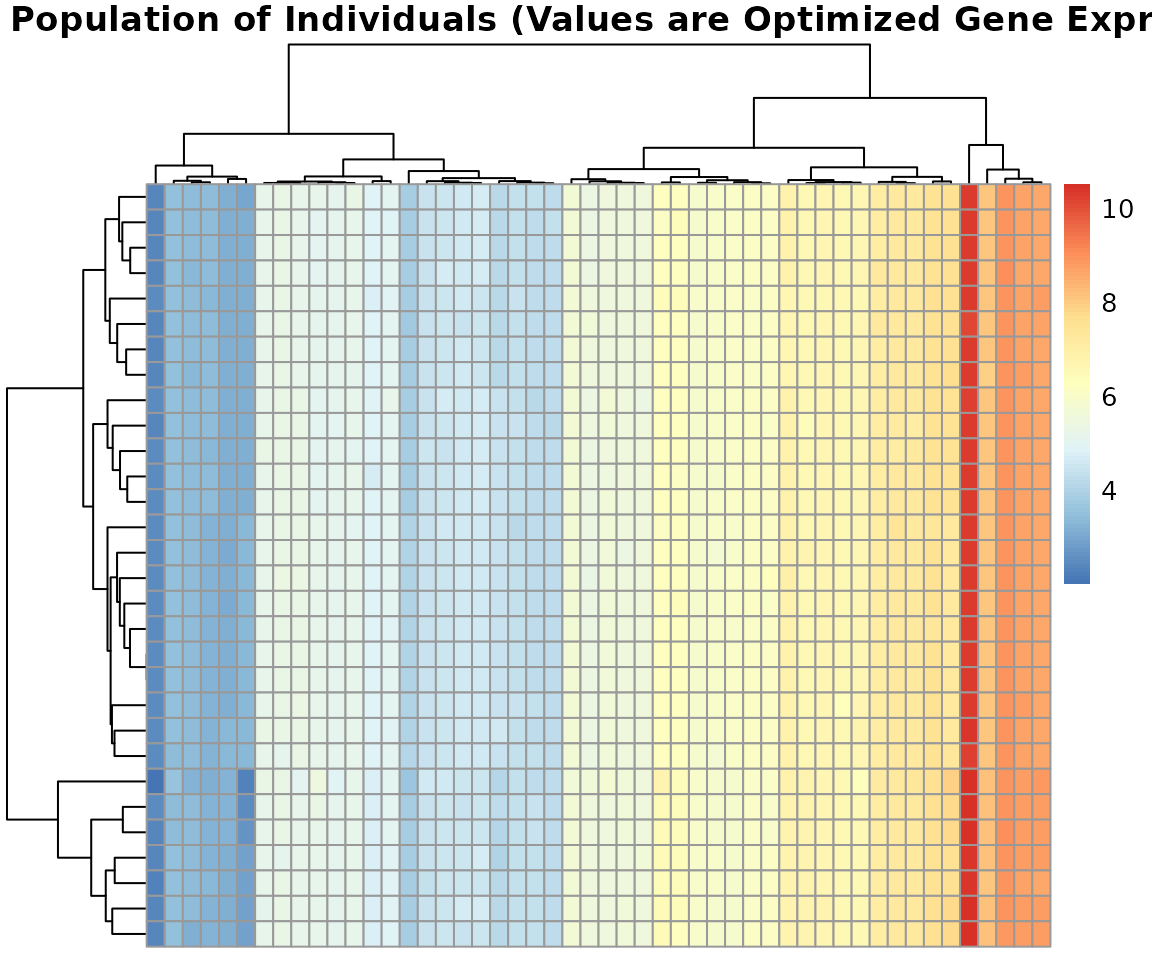
4.2 Gene Selection Frequency
A key application is gene signature selection. We can identify which genes the algorithm consistently preserved (i.e., maintained a non-zero value) across the final population.
# Calculate the mean frequency of non-zero values per gene (column)
gene_selection_freq <- colMeans(result$population != 0)
gene_selection_df <- data.frame(
    Gene = rownames(genomic_data),
    Frequency = gene_selection_freq
)

# Plotting the frequency
ggplot(gene_selection_df, aes(x = Gene, y = Frequency)) +
    geom_bar(stat = "identity", fill = "#D55E00") +
    labs(x = "Gene", y = "Selection Frequency (Non-Zero)",
         title = "Frequency of Gene Selection in Final Population") +
    theme_minimal(base_size = 12) +
    theme(axis.text.x = element_text(angle = 90, hjust = 1))
Genes with high selection frequency (approaching 1.0) represent the core
“signature” identified by the GA that optimally balances expression
difference and sparsity. In this example, we observe high frequency for
the
Genes with high selection frequency (approaching 1.0) represent the core
“signature” identified by the GA that optimally balances expression
difference and sparsity. In this example, we observe high frequency for
the Gene1 through Gene10 region, which matches
our simulated differentially expressed genes.
5. Advanced Feature: Network Constraint
The BioGA’s mutation operator can be constrained by a
gene-gene interaction network
().
This allows the search to prioritize biologically plausible changes,
reducing the mutation magnitude for genes that are highly connected. We
demonstrate how the mutation_cpp function handles external
network information.
# 1. Create a dummy network matrix (e.g., co-expression or regulatory links)
network_mat <- matrix(runif(n_genes^2, 0, 0.5), nrow = n_genes)
diag(network_mat) <- 0 # No self-loops

# Use the final population as a starting point for mutation
pop_to_mutate <- result$population

mutated_with_net <- mutation_cpp(
    population = pop_to_mutate,
    mutation_rate = 0.1,
    iteration = 10,
    max_iterations = 50,
    network = network_mat # Injecting the network constraint
)

pheatmap(mutated_with_net,
    main = "Population After Mutation with Network Constraint",
    show_rownames = FALSE, show_colnames = FALSE)
When a network is provided, the operator uses the expression , mathematically imposing that changes are dampened for key network hub genes.
Summary
The practical application:
- Simulated and visualized a multi-class genomic dataset.
- Executed the multi-objective GA with defined weights for data fidelity and sparsity.
- Provided a robust method for tracking and visualizing fitness convergence.
- Analyzed the final population for diversity and identified the optimal gene signature subset.
Further Customization
To apply BioGA to your research:
-
Real Data: Replace
genomic_datawith your own RNA-seq, microarrays, or proteomics data matrix. - Custom Objectives: Extend the multiple objectives by including clinical data (e.g., survival time, drug response) or external scores (e.g., literature scores) to guide the evolution.
-
Network Integration: Define a meaningful adjacency
matrix for
networkbased on databases like STRING or pre-computed co-expression to ensure biological relevance during mutation.
Performance Tip
For extremely large datasets (high or high ):
Use
RcppParallel::setThreadOptions(numThreads = N)before runningbioga_main_cppto explicitly control CPU thread usage and maximize parallel processing performance.
Session Info
sessioninfo::session_info()
#> ─ Session info ───────────────────────────────────────────────────────────────
#>  setting  value
#>  version  R version 4.5.2 (2025-10-31)
#>  os       Ubuntu 24.04.3 LTS
#>  system   x86_64, linux-gnu
#>  ui       X11
#>  language en
#>  collate  C.UTF-8
#>  ctype    C.UTF-8
#>  tz       UTC
#>  date     2025-12-04
#>  pandoc   3.1.11 @ /opt/hostedtoolcache/pandoc/3.1.11/x64/ (via rmarkdown)
#>  quarto   NA
#>
#> ─ Packages ───────────────────────────────────────────────────────────────────
#>  package              * version    date (UTC) lib source
#>  abind                  1.4-8      2024-09-12 [1] RSPM
#>  animation              2.8        2025-08-26 [1] RSPM
#>  assertthat             0.2.1      2019-03-21 [1] RSPM
#>  backports              1.5.0      2024-05-23 [1] RSPM
#>  Biobase                2.70.0     2025-10-29 [1] Bioconduc~
#>  BiocGenerics           0.56.0     2025-10-29 [1] Bioconduc~
#>  BiocManager            1.30.27    2025-11-14 [1] RSPM
#>  BiocParallel           1.44.0     2025-10-29 [1] Bioconduc~
#>  BiocStyle              2.38.0     2025-10-29 [1] Bioconduc~
#>  biocViews              1.78.0     2025-10-29 [1] Bioconduc~
#>  BioGA                * 0.99.17    2025-12-04 [1] local
#>  bitops                 1.0-9      2024-10-03 [1] RSPM
#>  bookdown               0.45       2025-10-03 [1] RSPM
#>  broom                  1.0.10     2025-09-13 [1] RSPM
#>  bslib                  0.9.0      2025-01-30 [1] RSPM
#>  cachem                 1.1.0      2024-05-16 [1] RSPM
#>  car                    3.1-3      2024-09-27 [1] RSPM
#>  carData                3.0-5      2022-01-06 [1] RSPM
#>  caret                  7.0-1      2024-12-10 [1] RSPM
#>  caretEnsemble          4.0.1      2024-09-12 [1] RSPM
#>  checkmate              2.3.3      2025-08-18 [1] RSPM
#>  class                  7.3-23     2025-01-01 [3] CRAN (R 4.5.2)
#>  cli                    3.6.5      2025-04-23 [1] RSPM
#>  codetools              0.2-20     2024-03-31 [3] CRAN (R 4.5.2)
#>  data.table             1.17.8     2025-07-10 [1] RSPM
#>  DelayedArray           0.36.0     2025-10-29 [1] Bioconduc~
#>  desc                   1.4.3      2023-12-10 [1] RSPM
#>  digest                 0.6.39     2025-11-19 [1] RSPM
#>  doParallel             1.0.17     2022-02-07 [1] RSPM
#>  dplyr                * 1.1.4      2023-11-17 [1] RSPM
#>  evaluate               1.0.5      2025-08-27 [1] RSPM
#>  farver                 2.1.2      2024-05-13 [1] RSPM
#>  fastmap                1.2.0      2024-05-15 [1] RSPM
#>  foreach                1.5.2      2022-02-02 [1] RSPM
#>  Formula                1.2-5      2023-02-24 [1] RSPM
#>  fs                     1.6.6      2025-04-12 [1] RSPM
#>  future                 1.68.0     2025-11-17 [1] RSPM
#>  future.apply           1.20.0     2025-06-06 [1] RSPM
#>  generics               0.1.4      2025-05-09 [1] RSPM
#>  GenomicRanges          1.62.0     2025-10-29 [1] Bioconduc~
#>  GEOquery               2.78.0     2025-10-29 [1] Bioconduc~
#>  ggplot2              * 4.0.1      2025-11-14 [1] RSPM
#>  ggpubr                 0.6.2      2025-10-17 [1] RSPM
#>  ggsignif               0.6.4      2022-10-13 [1] RSPM
#>  glmnet                 4.1-10     2025-07-17 [1] RSPM
#>  globals                0.18.0     2025-05-08 [1] RSPM
#>  glue                   1.8.0      2024-09-30 [1] RSPM
#>  gower                  1.0.2      2024-12-17 [1] RSPM
#>  graph                  1.88.0     2025-10-29 [1] Bioconduc~
#>  gridExtra              2.3        2017-09-09 [1] RSPM
#>  gtable                 0.3.6      2024-10-25 [1] RSPM
#>  hardhat                1.4.2      2025-08-20 [1] RSPM
#>  hms                    1.1.4      2025-10-17 [1] RSPM
#>  htmltools              0.5.8.1    2024-04-04 [1] RSPM
#>  htmlwidgets            1.6.4      2023-12-06 [1] RSPM
#>  iml                    0.11.4     2025-02-24 [1] RSPM
#>  ipred                  0.9-15     2024-07-18 [1] RSPM
#>  IRanges                2.44.0     2025-10-29 [1] Bioconduc~
#>  iterators              1.0.14     2022-02-05 [1] RSPM
#>  jquerylib              0.1.4      2021-04-26 [1] RSPM
#>  jsonlite               2.0.0      2025-03-27 [1] RSPM
#>  km.ci                  0.5-6      2022-04-06 [1] RSPM
#>  KMsurv                 0.1-6      2025-05-20 [1] RSPM
#>  knitr                  1.50       2025-03-16 [1] RSPM
#>  labeling               0.4.3      2023-08-29 [1] RSPM
#>  lattice                0.22-7     2025-04-02 [3] CRAN (R 4.5.2)
#>  lava                   1.8.2      2025-10-30 [1] RSPM
#>  lifecycle              1.0.4      2023-11-07 [1] RSPM
#>  lime                   0.5.3      2022-08-19 [1] RSPM
#>  limma                  3.66.0     2025-10-29 [1] Bioconduc~
#>  listenv                0.10.0     2025-11-02 [1] RSPM
#>  lubridate              1.9.4      2024-12-08 [1] RSPM
#>  magrittr               2.0.4      2025-09-12 [1] RSPM
#>  MASS                   7.3-65     2025-02-28 [3] CRAN (R 4.5.2)
#>  Matrix                 1.7-4      2025-08-28 [3] CRAN (R 4.5.2)
#>  MatrixGenerics         1.22.0     2025-10-29 [1] Bioconduc~
#>  matrixStats            1.5.0      2025-01-07 [1] RSPM
#>  Metrics                0.1.4      2018-07-09 [1] RSPM
#>  ModelMetrics           1.2.2.2    2020-03-17 [1] RSPM
#>  mvtnorm                1.3-3      2025-01-10 [1] RSPM
#>  nlme                   3.1-168    2025-03-31 [3] CRAN (R 4.5.2)
#>  nnet                   7.3-20     2025-01-01 [3] CRAN (R 4.5.2)
#>  numDeriv               2016.8-1.1 2019-06-06 [1] RSPM
#>  parallelly             1.45.1     2025-07-24 [1] RSPM
#>  patchwork              1.3.2      2025-08-25 [1] RSPM
#>  pec                    2025.06.24 2025-07-24 [1] RSPM
#>  pheatmap             * 1.0.13     2025-06-05 [1] RSPM
#>  pillar                 1.11.1     2025-09-17 [1] RSPM
#>  pkgconfig              2.0.3      2019-09-22 [1] RSPM
#>  pkgdown                2.2.0      2025-11-06 [1] any (@2.2.0)
#>  plyr                   1.8.9      2023-10-02 [1] RSPM
#>  pROC                   1.19.0.1   2025-07-31 [1] RSPM
#>  prodlim                2025.04.28 2025-04-28 [1] RSPM
#>  purrr                  1.2.0      2025-11-04 [1] RSPM
#>  R6                     2.6.1      2025-02-15 [1] RSPM
#>  ragg                   1.5.0      2025-09-02 [1] RSPM
#>  randomForest           4.7-1.2    2024-09-22 [1] RSPM
#>  RBGL                   1.86.0     2025-10-29 [1] Bioconduc~
#>  RColorBrewer           1.1-3      2022-04-03 [1] RSPM
#>  Rcpp                   1.1.0      2025-07-02 [1] RSPM
#>  RcppParallel           5.1.11-1   2025-08-27 [1] RSPM
#>  RCurl                  1.98-1.17  2025-03-22 [1] RSPM
#>  readr                  2.1.6      2025-11-14 [1] RSPM
#>  recipes                1.3.1      2025-05-21 [1] RSPM
#>  rentrez                1.2.4      2025-06-11 [1] RSPM
#>  reshape2               1.4.5      2025-11-12 [1] RSPM
#>  rlang                  1.1.6      2025-04-11 [1] RSPM
#>  rmarkdown              2.30       2025-09-28 [1] RSPM
#>  rpart                  4.1.24     2025-01-07 [3] CRAN (R 4.5.2)
#>  rstatix                0.7.3      2025-10-18 [1] RSPM
#>  RUnit                  0.4.33.1   2025-06-17 [1] RSPM
#>  S4Arrays               1.10.1     2025-12-01 [1] Bioconduc~
#>  S4Vectors              0.48.0     2025-10-29 [1] Bioconduc~
#>  S7                     0.2.1      2025-11-14 [1] RSPM
#>  sass                   0.4.10     2025-04-11 [1] RSPM
#>  scales                 1.4.0      2025-04-24 [1] RSPM
#>  Seqinfo                1.0.0      2025-10-29 [1] Bioconduc~
#>  sessioninfo          * 1.2.3      2025-02-05 [1] RSPM
#>  shape                  1.4.6.1    2024-02-23 [1] RSPM
#>  SparseArray            1.10.4     2025-12-01 [1] Bioconduc~
#>  statmod                1.5.1      2025-10-09 [1] RSPM
#>  stringi                1.8.7      2025-03-27 [1] RSPM
#>  stringr                1.6.0      2025-11-04 [1] RSPM
#>  SummarizedExperiment   1.40.0     2025-10-29 [1] Bioconduc~
#>  survival               3.8-3      2024-12-17 [3] CRAN (R 4.5.2)
#>  survminer              0.5.1      2025-09-02 [1] RSPM
#>  survMisc               0.5.6      2022-04-07 [1] RSPM
#>  systemfonts            1.3.1      2025-10-01 [1] RSPM
#>  textshaping            1.0.4      2025-10-10 [1] RSPM
#>  tibble                 3.3.0      2025-06-08 [1] RSPM
#>  tidyr                  1.3.1      2024-01-24 [1] RSPM
#>  tidyselect             1.2.1      2024-03-11 [1] RSPM
#>  timechange             0.3.0      2024-01-18 [1] RSPM
#>  timeDate               4051.111   2025-10-17 [1] RSPM
#>  timereg                2.0.7      2025-08-18 [1] RSPM
#>  timeROC                0.4        2019-12-18 [1] RSPM
#>  tzdb                   0.5.0      2025-03-15 [1] RSPM
#>  vctrs                  0.6.5      2023-12-01 [1] RSPM
#>  withr                  3.0.2      2024-10-28 [1] RSPM
#>  xfun                   0.54       2025-10-30 [1] RSPM
#>  xgboost                1.7.11.1   2025-05-15 [1] RSPM
#>  XML                    3.99-0.20  2025-11-08 [1] RSPM
#>  xml2                   1.5.1      2025-12-01 [1] RSPM
#>  xtable                 1.8-4      2019-04-21 [1] RSPM
#>  XVector                0.50.0     2025-10-29 [1] Bioconduc~
#>  yaml                   2.3.11     2025-11-28 [1] RSPM
#>  zoo                    1.8-14     2025-04-10 [1] RSPM
#>
#>  [1] /home/runner/work/_temp/Library
#>  [2] /opt/R/4.5.2/lib/R/site-library
#>  [3] /opt/R/4.5.2/lib/R/library
#>  * ── Packages attached to the search path.
#>
#> ──────────────────────────────────────────────────────────────────────────────
```