GeneScout: De Novo Small ORF Discovery

Abstract

Hidden small open reading frames (sORFs) within non-coding genomic regions represent an underexplored layer of gene regulation and functional potential. Several Bioconductor/R packages, including Biostrings and coRdon, provide robust tools for sequence manipulation and codon usage bias analysis; however, these methods are primarily designed for annotated genes and assume prior knowledge of gene coordinates. Consequently, they are not optimized for the systematic exploration of large, unannotated genomic regions.

GeneScout addresses this methodological gap by enabling de novo sORF discovery directly from raw genomic sequences. The package implements sliding window–based entropy scanning, Shannon entropy estimation, and Kullback–Leibler divergence to quantify local codon usage bias without requiring GTF or GFF annotations. In addition, GeneScout supports comparative visualization of entropy profiles and integration with RNA-Seq data to prioritize biologically relevant candidates. By automating these analyses across large genomic intervals, GeneScout facilitates the identification of previously overlooked coding regions within non-coding DNA.

The problem: Even in well-studied genomes, large stretches of “junk” DNA actually contain small, hidden genes. These can be identified by looking for patterns in codon usage using entropy analysis.

In non-coding DNA, codons appear randomly (high entropy)
In real genes, organisms prefer specific codons (low entropy)

GeneScout provides tools to calculate codon usage profiles from known genes, scan large genomic regions with a sliding window, identify regions with low entropy (potential coding regions), and find candidate ORFs within those regions.

Installation

# install development version
devtools::install_github("danymukesha/GeneScout")

Quick start

Basic enthropy calculation

First, calculate codon frequencies and Shannon entropy for a sequence:

# Example sequence (biased codon usage)
sequence1 <- "ATGATGATGATGATGATGTTATTATTATTATTATTATTACGCCGCCGCCGCCGCC"

freqs <- calculate_codon_frequencies(sequence1)
print(head(freqs[freqs > 0]))

##       TTA       CGC       ATG 
## 0.3888889 0.2777778 0.3333333

entropy <- calculate_shannon_entropy(freqs)
print(paste("Shannon Entropy:", round(entropy, 3), "bits"))

## [1] "Shannon Entropy: 1.572 bits"

Create a reference profile

For de novo discovery, create a reference profile from known genes:

# Known gene sequences (would normally be from annotated genes)
known_genes <- c(
  "ATGATGATGATGCCGCCGCCGCCTTATTATTATTAG",
  "ATGCCGCCGCCGCCATTATTATTAATGTTTTTTTTT",
  "ATGTTTTTTTTTTTACGCCGCCGCCGCCGAGTAA"
)

# Create reference codon usage profile
ref_profile <- create_reference_profile(known_genes, method = "mean")
print(head(ref_profile[ref_profile > 0]))

##        CCA        CGA        GTA        TTA        CGC        TAG 
## 0.02777778 0.03030303 0.03030303 0.11363636 0.12121212 0.02777778

Sliding window scan

Perform a genome-wide scan to find regions matching the reference profile:

# Create a longer test sequence with embedded "gene-like" regions
test_sequence <- paste0(
  paste0(rep("ACGTACGTACGT", 30), collapse = ""),  # Random region
  "ATGATGATGATGCCGCCGCCGCCTTATTATTATTA",       # Embedded ORF
  paste0(rep("TGACTGACTGA", 30), collapse = ""), # Random region
  "ATGCCGCCGCCGCCATTATTATTAATGTTTTTTTTTTAG",   # Another ORF
  paste0(rep("GATCGATCGAT", 30), collapse = "") # Random region
)


# Scan with sliding window
scan_result <- sliding_window_scan(
  test_sequence,
  window_size = 150,
  step_size = 30,
  reference_profile = ref_profile
)

# View results
print(scan_result)

## GeneScout Sliding Window Scan Results
## =======================================
## Number of windows: 32 
## Sequence range: 1 - 1080 bp
## 
## Entropy Statistics:
##   Mean Shannon Entropy: 2.665 bits
##   Std. Dev. Shannon Entropy: 0.598 bits
##   Min Shannon Entropy: 1.999 bits
##   Max Shannon Entropy: 3.896 bits
## 
## KL Divergence Statistics:
##   Mean KL Divergence: 23.452 
##   Std. Dev. KL Divergence: 3.108

Detect Entropy Peaks

Identify regions with unusually low entropy:

# Detect peaks in entropy profile
peaks <- entropy_peak_detection(
  scan_result,
  metric = "shannon_entropy",
  method = "quantile",
  threshold = 0.1,
  min_peak_width = 3
)

print(peaks)

##   peak_id start_window end_window num_windows start_bp end_bp metric_value_mean
## 1       1            1          8           8        1    360          1.998846
##   metric_value_min
## 1         1.998846

Find candidate ORFs

Search for actual ORFs within the low-entropy peaks:

# Find candidate ORFs
candidates <- find_candidate_orfs(
  test_sequence,
  scan_result,
  peaks,
  min_orf_length = 60,
  start_codons = c("ATG"),
  stop_codons = c("TAA", "TAG", "TGA")
)

print(candidates)

## # A tibble: 0 × 0

Visualize results

Create plots to visualize entropy profiles and candidate ORFs:

# Plot entropy profile
plot_entropy_profile(scan_result, 
                     metric = "shannon_entropy",
                     highlight_threshold = TRUE)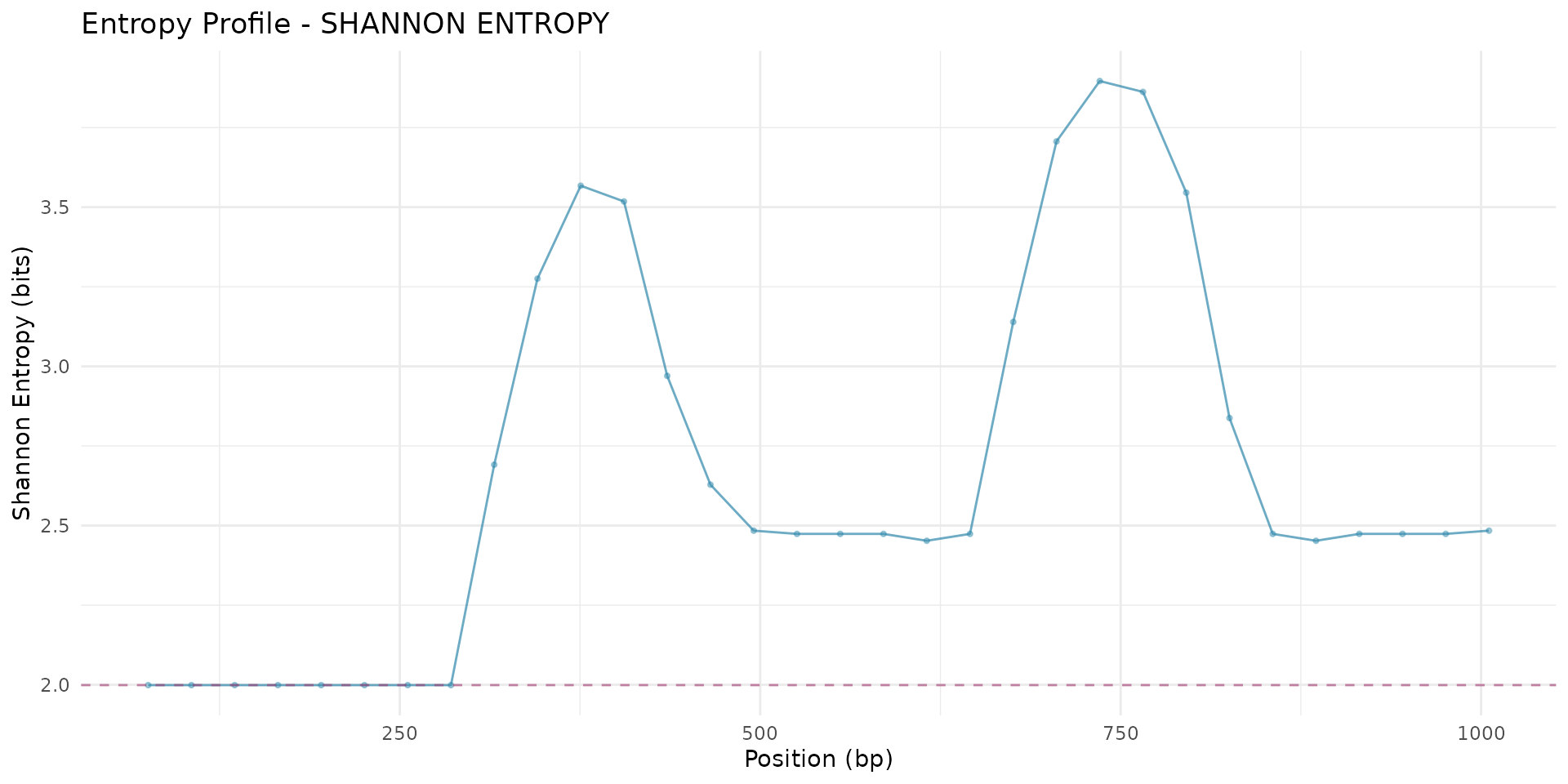

# Plot with peaks highlighted
plot_entropy_profile(scan_result, 
                     peaks = peaks,
                     metric = "shannon_entropy",
                     show_peaks = TRUE)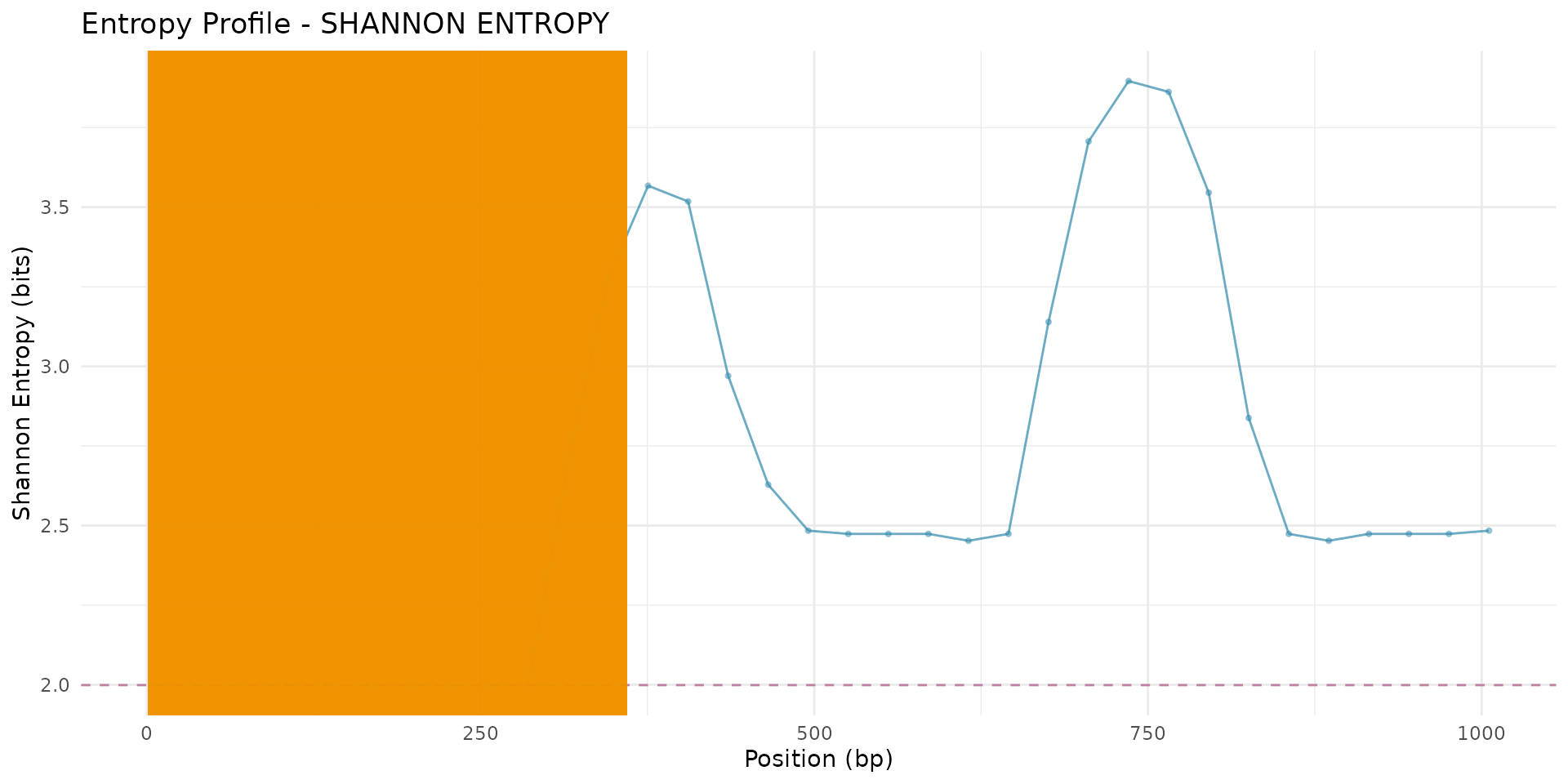

# Plot candidate ORFs
plot_candidate_orfs(scan_result, candidates, peaks, metric = "shannon_entropy")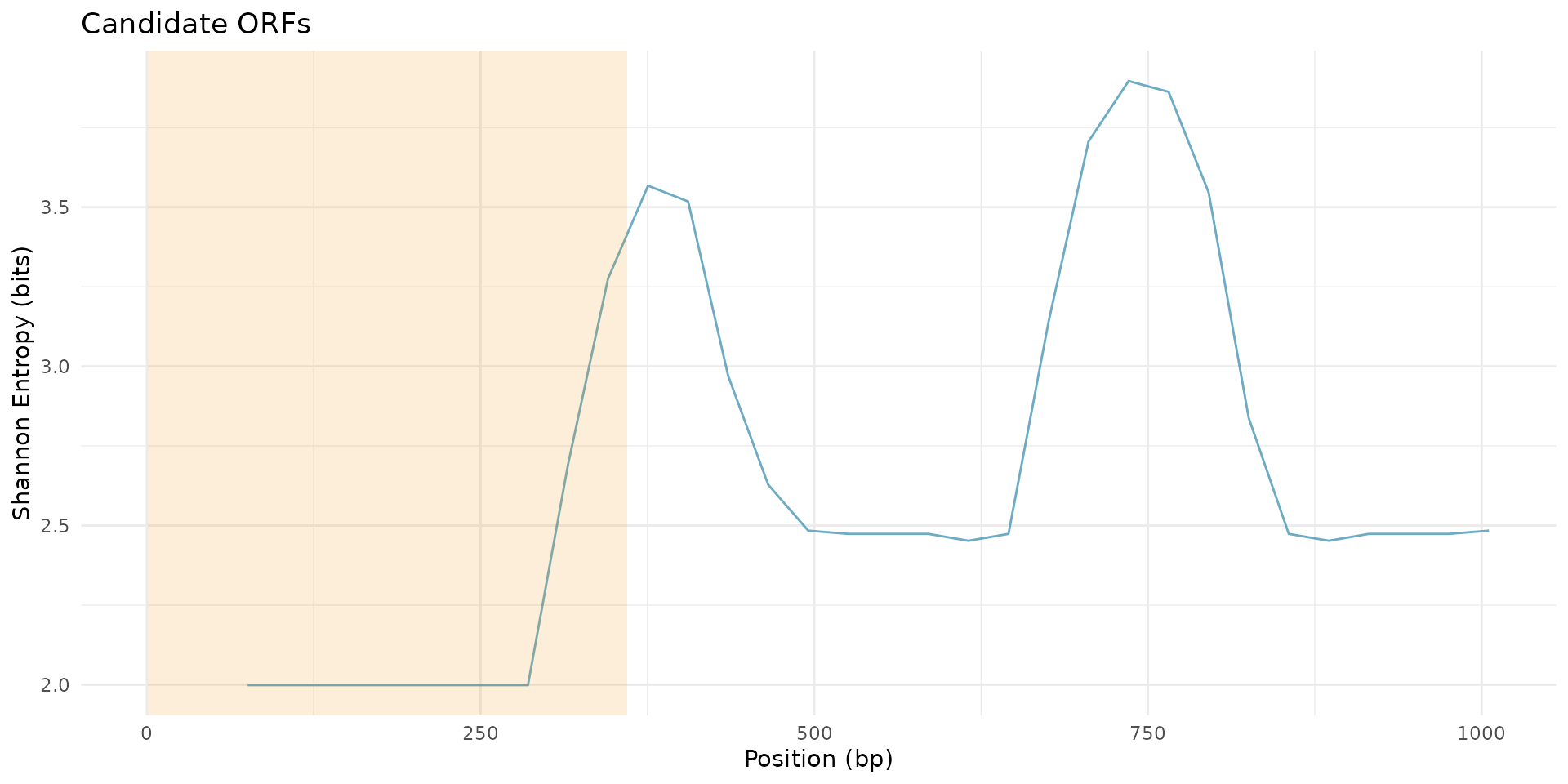

Advanced usage

Comparative analysis

Compare entropy profiles between different regions:

# Create two different sequences
# APOE coding region (simulated longer fragment for demo, ~4 kb)
seq_region1 <- paste0(
    "ATGGAGGAGCCGCAGTCAGATCCTAGCGTCGAGCAGGAGAGCTGCGGGAGGAGCGGAGGCTG",
    "GAGGCCGCGGAGGAGCTGGCGGAGGCGGAGGAGGCGGAGGAGCCGCGGAGGAGGAGGAGGAG",
    "GCCGCGGAGGAGGCGGAGGAGGAGGAGGAGGAGGAGGAGGAGGAGGAGGAGGAGGAGGAGGA",
    "GAGGAGGAGGAGGAGGAGGAGGAGGAGGAGGAGGAGGAGGAGGAGGAGGAGGAGGAGGAGGA",
    "GAGGAGGAGGAGGAGGAGGAGGAGGAGGAGGAGGAGGAGGAGGAGGAGGAGGAGGAGGAGGA",
    "GCCGCGGAGGAGGCGGAGGAGGAGGAGGAGGAGGAGGAGGAGGAGGAGGAGGAGGAGGAGGA",
    "GAGGAGGAGGAGGAGGAGGAGGAGGAGGAGGAGGAGGAGGAGGAGGAGGAGGAGGAGGAGGA",
    "GAGGAGGAGGAGGAGGAGGAGGAGGAGGAGGAGGAGGAGGAGGAGGAGGAGGAGGAGGAGGA",
    "GAGGAGGAGGAGGAGGAGGAGGAGGAGGAGGAGGAGGAGGAGGAGGAGGAGGAGGAGGAGGA"
)
# Random-like region from chr19 (simulated, ~4 kb)
seq_region2 <- paste0(
    "GCGTACGTAGCTAGCGTAGCTACGTAGCTAGCTGACGATCAGTGCTAGCTAGCTAGCGTAC",
    "GATCGATCGATCGTAGCTAGCTAGCTAGCGTACGATCGATCGTAGCTAGCTAGCTGACGAT",
    "CGTAGCTAGCTGACGATCGTACGATGCTAGCTAGCTGATCGTAGCTAGCTAGCTAGCGTAC",
    "GATCGATCGTAGCTAGCTAGCTGACGATCGTAGCTAGCTGACGATCGTACGATGCTAGCTA",
    "TACGATCGATCGATCGTAGCTAGCTAGCTAGCGTACGATCGATCGTAGCTAGCTAGCTGAC",
    "GATCGTAGCTAGCTGACGATCGTACGATGCTAGCTAGCTGATCGTAGCTAGCTAGCTAGCG",
    "TACGATCGATCGTAGCTAGCTAGCTGACGATCGTAGCTAGCTGACGATCGTACGATGCTAG",
    "CTATACGATCGATCGATCGTAGCTAGCTAGCTAGCGTACGATCGATCGTAGCTAGCTAGCT",
    "GACGATCGTAGCTAGCTGACGATCGTACGATGCTAGCTAGCTGATCGTAGCTAGCTAGCTA"
)

# Scan both regions
result1 <- sliding_window_scan(seq_region1, window_size = 100, step_size = 20)
result2 <- sliding_window_scan(seq_region2, window_size = 100, step_size = 20)

# Compare profiles
compare_entropy_profiles(result1, result2, 
                         labels = c("Gene-like region", "Random region"))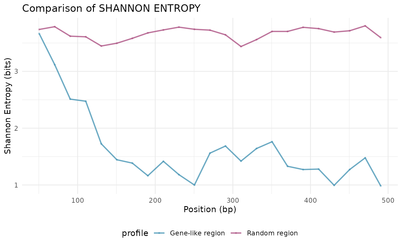

Working with genomes

For large genomes, process chromosome by chromosome:

# Read genome FASTA file (https://parasite.wormbase.org/index.html)
genome <- read_fasta("../inst/extdata/acanthocheilonema_viteae.PRJEB1697.WBPS19.genomic.fa")

# Extract known genes from GTF annotation file
known_genes <- extract_known_genes(
  gtf_file = "../inst/extdata/acanthocheilonema_viteae.PRJEB1697.WBPS19.canonical_geneset.gtf",
  genome_fasta = "../inst/extdata/acanthocheilonema_viteae.PRJEB1697.WBPS19.genomic.fa",
  feature_type = "gene",
  min_length = 150,
  max_genes = 1000
)

# Create reference profile from extracted genes
ref_profile <- create_reference_profile(known_genes[1:11])

# Process one chromosome
chr_name <- names(genome)[1]
chr_sequence <- as.character(genome[1])

# Scan chromosome
chr_scan <- sliding_window_scan(
  chr_sequence,
  window_size = 300,
  step_size = 30,
  reference_profile = ref_profile
)

# Detect peaks and find ORFs
peaks <- entropy_peak_detection(chr_scan, threshold = 0.05)
candidates <- find_candidate_orfs(chr_sequence, chr_scan, peaks)

# Save results
write.csv(candidates, paste0("candidates_", chr_name, ".csv"))

Theory behind GeneScout

Shannon enthropy

Shannon entropy measures the “surprise” or randomness of data:

$H = -\sum_{i=1}^{64} P(i) \log_2 P(i)$

Where $P(i)$ is the frequency of codon $i$ .

High entropy (~6 bits): Random codon usage (non-coding DNA)
Low entropy (~3-4 bits): Biased codon usage (potential gene)

Kullback-Leibler divergance

KL divergence measures how one distribution differs from another:

$D_{KL}(P \| Q) = \sum_{i} P(i) \log_2 \left( \frac{P(i)}{Q(i)} \right)$

Where $P(i)$ is the observed frequency and $Q(i)$ is the reference frequency.

High KL: Window differs from organism’s typical codon usage
Low KL: Window matches organism’s typical codon usage

Effective Number of Codons (ENC)

ENC is another measure of codon usage bias:

# Calculate ENC for different sequences
seq_uniform <- paste(rep(c("ATG", "TTT", "CCC", "GGG", "AAA", "TTT"), 10), 
                     collapse = "")
seq_biased <- paste(rep("ATG", 60), collapse = "")

freqs_uniform <- calculate_codon_frequencies(seq_uniform)
freqs_biased <- calculate_codon_frequencies(seq_biased)

enc_uniform <- calculate_enc(freqs_uniform)
enc_biased <- calculate_enc(freqs_biased)

print(paste("Uniform sequence ENC:", round(enc_uniform, 2)))

## [1] "Uniform sequence ENC: 16"

print(paste("Biased sequence ENC:", round(enc_biased, 2)))

## [1] "Biased sequence ENC: 2"

ENC ranges from 20 (extreme bias) to 61 (no bias).

Parameter tuning

Window size

The choice of window size affects sensitivity:

Small windows (50-100 bp): Higher sensitivity, more noise
Large windows (300-500 bp): More stable, may miss small ORFs

# Compare different window sizes
windows <- c(100, 150, 300)

results <- lapply(windows, function(ws) {
  sliding_window_scan(test_sequence, window_size = ws, step_size = 30)
})

Step size

Step size determines resolution:

Small step (10-20 bp): Fine-grained scan, slower
Large step (30-50 bp): Faster scan, may miss features

Threshold selection

Use different methods to set entropy thresholds:

# Quantile-based threshold
peaks_quantile <- entropy_peak_detection(
  scan_result, 
  method = "quantile", 
  threshold = 0.1
)

# Standard deviation-based threshold
peaks_sd <- entropy_peak_detection(
  scan_result, 
  method = "sd", 
  threshold = 1.5
)

Integration with RNA-Seq

For validation, integrate with RNA-seq expression data:

# Load RNA-seq coverage data
coverage <- readRDS("rnaseq_coverage.rds")

# Add expression information to candidates
candidates_with_expr <- dplyr::mutate(candidates,
  mean_coverage = sapply(1:nrow(candidates), function(i) {
    mean(coverage[candidates$start[i]:candidates$end[i]])
  })
)

# Filter by expression
expressed_candidates <- dplyr::filter(
  candidates_with_expr,
  mean_coverage > 5
)

Performance consideration

For large genomes:

Process by chromosome: Avoid loading entire genome into memory
Use parallel processing: Scan different chromosomes in parallel
Optimize parameters: Larger step sizes reduce computation
Filter early: Exclude low-complexity regions before scanning

# Parallel scanning example
library(parallel)
library(foreach)
library(doParallel)

cl <- makeCluster(detectCores() - 1)
registerDoParallel(cl)

results <- foreach(chr = chromosome_names) %dopar% {
  chr_seq <- as.character(genome[chr])
  sliding_window_scan(chr_seq, window_size = 300, step_size = 30)
}

stopCluster(cl)

References

Wright, F. (1990). The ‘effective number of codons’ used in a gene. Gene, 87(1), 23-29.
Sharp, P. M., & Li, W. H. (1987). The codon Adaptation Index-a measure of directional synonymous codon usage bias, and its potential applications. Nucleic Acids Research, 15(3), 1281-1295.

Session information

sessionInfo()

## R version 4.5.2 (2025-10-31)
## Platform: x86_64-pc-linux-gnu
## Running under: Ubuntu 24.04.3 LTS
## 
## Matrix products: default
## BLAS:   /usr/lib/x86_64-linux-gnu/openblas-pthread/libblas.so.3 
## LAPACK: /usr/lib/x86_64-linux-gnu/openblas-pthread/libopenblasp-r0.3.26.so;  LAPACK version 3.12.0
## 
## locale:
##  [1] LC_CTYPE=C.UTF-8       LC_NUMERIC=C           LC_TIME=C.UTF-8       
##  [4] LC_COLLATE=C.UTF-8     LC_MONETARY=C.UTF-8    LC_MESSAGES=C.UTF-8   
##  [7] LC_PAPER=C.UTF-8       LC_NAME=C              LC_ADDRESS=C          
## [10] LC_TELEPHONE=C         LC_MEASUREMENT=C.UTF-8 LC_IDENTIFICATION=C   
## 
## time zone: UTC
## tzcode source: system (glibc)
## 
## attached base packages:
## [1] stats     graphics  grDevices utils     datasets  methods   base     
## 
## other attached packages:
## [1] GeneScout_0.99.0 BiocStyle_2.38.0
## 
## loaded via a namespace (and not attached):
##  [1] SummarizedExperiment_1.40.0 gtable_0.3.6               
##  [3] rjson_0.2.23                xfun_0.56                  
##  [5] bslib_0.10.0                ggplot2_4.0.1              
##  [7] lattice_0.22-7              Biobase_2.70.0             
##  [9] vctrs_0.7.1                 tools_4.5.2                
## [11] bitops_1.0-9                generics_0.1.4             
## [13] stats4_4.5.2                curl_7.0.0                 
## [15] parallel_4.5.2              tibble_3.3.1               
## [17] pkgconfig_2.0.3             Matrix_1.7-4               
## [19] RColorBrewer_1.1-3          cigarillo_1.0.0            
## [21] S7_0.2.1                    desc_1.4.3                 
## [23] S4Vectors_0.48.0            lifecycle_1.0.5            
## [25] compiler_4.5.2              farver_2.1.2               
## [27] stringr_1.6.0               Rsamtools_2.26.0           
## [29] textshaping_1.0.4           Biostrings_2.78.0          
## [31] Seqinfo_1.0.0               codetools_0.2-20           
## [33] htmltools_0.5.9             sass_0.4.10                
## [35] RCurl_1.98-1.17             yaml_2.3.12                
## [37] pillar_1.11.1               pkgdown_2.2.0              
## [39] crayon_1.5.3                jquerylib_0.1.4            
## [41] tidyr_1.3.2                 BiocParallel_1.44.0        
## [43] DelayedArray_0.36.0         cachem_1.1.0               
## [45] abind_1.4-8                 tidyselect_1.2.1           
## [47] digest_0.6.39               stringi_1.8.7              
## [49] dplyr_1.1.4                 purrr_1.2.1                
## [51] restfulr_0.0.16             bookdown_0.46              
## [53] labeling_0.4.3              fastmap_1.2.0              
## [55] grid_4.5.2                  SparseArray_1.10.8         
## [57] cli_3.6.5                   magrittr_2.0.4             
## [59] S4Arrays_1.10.1             XML_3.99-0.20              
## [61] withr_3.0.2                 scales_1.4.0               
## [63] rmarkdown_2.30              XVector_0.50.0             
## [65] httr_1.4.7                  matrixStats_1.5.0          
## [67] ragg_1.5.0                  evaluate_1.0.5             
## [69] knitr_1.51                  GenomicRanges_1.62.1       
## [71] IRanges_2.44.0              BiocIO_1.20.0              
## [73] rtracklayer_1.70.1          rlang_1.1.7                
## [75] glue_1.8.0                  BiocManager_1.30.27        
## [77] BiocGenerics_0.56.0         jsonlite_2.0.0             
## [79] R6_2.6.1                    MatrixGenerics_1.22.0      
## [81] GenomicAlignments_1.46.0    systemfonts_1.3.1          
## [83] fs_1.6.6

Dany Mukesha

2026-01-28